Download

1 / 15
150 likes | 225 Views
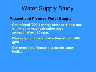
Water Supply Study. Present and Planned Water Supply Operational (2001) spring water bottling plant, with groundwater extraction rates approximating 125 gpm. Planned groundwater extraction of up to 400 gpm. Concerns about impacts to nearby water bodies. Critical Prediction.

E N D
Water Supply Study • Present and Planned Water Supply • Operational (2001) spring water bottling plant, with groundwater extraction rates approximating 125 gpm. • Planned groundwater extraction of up to 400 gpm. • Concerns about impacts to nearby water bodies.
Critical Prediction Calculate changes in Surface-Water Flows, Wetland and Lake Levels from Constant Production of 400 gpm
Regional Model Design Selected Code MODFLOW2000 Model Summary 4 layers Conductivity zones derived from regional/local geologic studies Variable recharge derived from published regression analysis Study Area
Local Model Area Groundwater Flow Pumping Center Impoundment Spring Outfall Stream
Shortcomings in Problem Formulation • Modeling Tool – Use of River Package • Inability to realistically represent changes in streams, wetlands, and lakes. • Inability to explicitly represent the impoundment-overflow
Stream Impoundment Culvert Discharge Stream
Revised Problem Formulation • Digitized stream intersections and topo maps to assign MODFLOW Drain/River - revised during calibration. • Impoundment and nearby lakes represented with Lake Package (Merritt and Konikow, 2000); outflow from impoundment explicitly modeled. • Four wetlands with standing water modeled with Lake Package to explicitly simulate wetland water levels. • Stream simulated using MODFLOW Drain Package plus Impoundment outflow. • Regional river comprises down gradient drainage center.
Model Calibration • Calibration Strategy • Steady-state calibration to water levels in 48 wells, baseflow in five creeks, and lake levels in five lakes. • Transient calibration to drawdowns from long-term (72 hour) pumping test - one dozen wells with time-series drawdown data • Prior information used to establish total transmissivity as ‘soft’ information during steady-state calibration • Approx. 40 parameters – step-wise reduction using tied/untied parameters as calibration progressed • PEST used in parallel across four 1.8GHz processors
PEST Pre-Post Processing • Advantages over GUI or ‘prompt’ Execution • Ability to assess progress with every run • Ability to re-parameterize (tie, hold, transform, scale, prior, regularize) model without ‘rebuild’ • Ability to alter run type with one (or two) quick Control File modifications – Forward run, Estimation, Regularization, and Prediction
program fluxes c Read output from MF2K Lak package modified by Mark Kuhl, to sum c baseflows over target reaches and write to single file for use c as PEST targets. c General declarations parameter(ncol=243,nrow=164,nlay=4) implicit double precision (c,d,r,g,s,m, b) dimension riv(:,:), drn(:,:), iriv_rch(:,:) , idrn_rch(:,:) integer kper, kstp, jj, i, j, k, idrn_rch, iriv_rch, nriv, idum c Files produced by MKUHL's MODFLOW Package character*20 drnfile, rivfile character*23 lakfile c Output file from this program for PEST character*12 pestout c Specific Target Names c 1: COLE_CREEK: Drain Reach 1 c 2: GILBERT_CREEK: Drain Reach 2, River Reach 2 c 3: DEAD_STREAM: Drain Reach 3 c 4: BURDON_CREEK: River Reach 3 c 5: MUSKEGON_RIVER: River Reach 4 + SUMMED COMPONENTS allocatable riv, drn, idrn_rch, iriv_rch allocate(riv(ncol,nrow),drn(ncol,nrow), idrn_rch(ncol,nrow), + iriv_rch(ncol,nrow)) drnfile='drain_cell_flows.dat' rivfile='river_cell_flows.dat' lakfile='lake_flow_and_level.dat' pestout='pestout.dat' idrn_rch=0 iriv_rch=0 c======================================================================= c MAIN PROGRAM START c======================================================================= c Read drain flows: KPER, KSTP ,R, C, Q (L^3/T) Open(1,file=drnfile) Read(1,*) Do jj=1,20000 c Use drntemp to account for multiple reaches in one cell drntemp=0. read(1,1,end=991) kper, kstp, i, j, drntemp drn(j,i) = drn(j,i)+drntemp End do 991 Close(1) c Read river flows: KPER, KSTP ,R, C, Q (L^3/T) Open(1,file=rivfile) Read(1,*) Do jj=1,20000 c Use rivtemp to account for multiple reaches in one cell rivtemp=0. read(1,1,end=992) kper, kstp, i, j, rivtemp riv(j,i) = riv(j,i) + rivtemp End do 992 Close(1) c Read Osprey Lake outflows, and stages for the five simulated lakes Open(1,file=lakfile) Read(1,*) sprey_out, sL1, sL2 Close(1) c======================================================================= c 1: COLE CREEK - Comprises drains ONLY: SG-103 c======================================================================= c Drain flows within COL-ROW range COLE_CREEK = 0. do i=1,nrow do j=1,ncol if (i.ge.21.and.i.le.121) then if (j.ge.16.and.j.le.144) then COLE_CREEK = COLE_CREEK + drn(j,i) idrn_rch(j,i) = 1 endif endif end do end do c Subtract flows which accumulate and go northwards at divide COLE_NORTH = 0. do i=1,nrow do j=1,ncol if (i.ge.32.and.i.le.47) then if (j.ge.42.and.j.le.49) then COLE_NORTH = COLE_NORTH + drn(j,i) idrn_rch(j,i) = 0 endif endif end do end do COLE_CREEK = COLE_CREEK - COLE_NORTH c======================================================================= c 2: GILBERT_CREEK - Comprises drains and rivers: SG-101 c======================================================================= c Drain flows within COL-ROW range GILBERT_DRAIN = 0. do i=1,nrow do j=1,ncol if (i.ge.16.and.i.le.96) then if (j.ge.166.and.j.le.211) then GILBERT_DRAIN = GILBERT_DRAIN + drn(j,i) idrn_rch(j,i) = 2 endif endif end do end do c River flows upgradient of drain delineation GILBERT_RIVER = 0. do i=1,nrow do j=1,ncol if (i.ge.4.and.i.le.15) then if (j.ge.16.and.j.le.210) then GILBERT_RIVER = GILBERT_RIVER + riv(j,i) iriv_rch(j,i) = 2 endif endif end do end do GILBERT_CREEK = GILBERT_DRAIN + GILBERT_RIVER write(*,*) GILBERT_DRAIN, GILBERT_RIVER c======================================================================= c 3: DEAD_STREAM - Comprises drains and Osprey Lake Outflow: SG-102 c======================================================================= c Drain flows within COL-ROW range DEAD_STREAM = 0. do i=1,nrow do j=1,ncol if (i.ge.97.and.i.le.113) then if (j.ge.175.and.j.le.204) then DEAD_STREAM = DEAD_STREAM + drn(j,i) idrn_rch(j,i) = 3 endif endif end do end do c Osprey Lake outflows: use NEGATIVE of Sprey_out as this is +ve DEAD_STREAM = DEAD_STREAM + (-SPREY_OUT) c======================================================================= c 4: BURDON_CREEK - Comprises rivers only: SG-104 c======================================================================= c River flows within COL-ROW range BURDON_CREEK = 0. do i=1,nrow do j=1,ncol if (i.ge.92.and.i.le.126) then if (j.ge.11.and.j.le.53) then BURDON_CREEK = BURDON_CREEK + riv(j,i) iriv_rch(j,i) = 3 endif endif end do end do c======================================================================= c 5: MUSKEGON_RIVER - All drainage contributing to tri-lakes: SG-105 c======================================================================= c Begin by summing all the components calculated above MUSKEGON_RIVER = 0. MUSKEGON_RIVER = COLE_CREEK + GILBERT_CREEK + DEAD_STREAM + + BURDON_CREEK Write(*,*) 'MUSKEGON TRIBS :', MUSKEGON_RIVER c Now account for river cells representing the main lakes, etc. do i=1,nrow do j=1,ncol if (i.ge.89.and.i.le.125) then if (j.ge.54.and.j.le.213) then MUSKEGON_RIVER = MUSKEGON_RIVER + riv(j,i) C if (riv(j,i).ne.0) then C write(*,*) j,i,riv(j,i) C end if iriv_rch(j,i) = 4 endif endif end do end do Write(*,*) 'MUSKEGON TRIBS + WEST RIVERS:', MUSKEGON_RIVER do i=1,nrow do j=1,ncol if (i.ge.126.and.i.le.128) then if (j.ge.197.and.j.le.211) then MUSKEGON_RIVER = MUSKEGON_RIVER + riv(j,i) iriv_rch(j,i) = 4 endif endif end do end do Write(*,*) 'MUSKEGON TRIBS + MID RIVERS :', MUSKEGON_RIVER do i=1,nrow do j=1,ncol if (i.ge.129.and.i.le.129) then if (j.ge.209.and.j.le.211) then MUSKEGON_RIVER = MUSKEGON_RIVER + riv(j,i) iriv_rch(j,i) = 4 endif endif end do end do Write(*,*) 'MUSKEGON TRIBS + ALL BODIES :', MUSKEGON_RIVER c======================================================================= c Write target data to single file for PEST c======================================================================= COLE_CREEK = (LOG10(-COLE_CREEK)) GILBERT_CREEK = (LOG10(-GILBERT_CREEK)) DEAD_STREAM = (LOG10(-DEAD_STREAM)) BURDON_CREEK = (LOG10(-BURDON_CREEK)) MUSKEGON_RIVER= (LOG10(-MUSKEGON_RIVER)) if (sprey_out.gt.0.) then Sprey_out = (LOG10(Sprey_out)) else sprey_out = 0. End if Open(1,file=pestout) Write(1,'(a30)') 'FLUX TARGET MODELED' Write(1,'(a19,e15.7)') 'COLE_CREEK :', COLE_CREEK Write(1,'(a19,e15.7)') 'GILBERT_CREEK :', GILBERT_CREEK Write(1,'(a19,e15.7)') 'DEAD_STREAM :', DEAD_STREAM Write(1,'(a19,e15.7)') 'BURDON_CREEK :', BURDON_CREEK Write(1,'(a19,e15.7)') 'MUSKEGON_RIVER :', MUSKEGON_RIVER Write(1,'(a19,e15.7)') 'OSPREY LAKE OUTFL :', Sprey_out Write(1,'(a19,e15.7)') 'OSPREY LAKE LEVEL :', sL1 Write(1,'(a19,e15.7)') 'LAKE 2 LEVEL :', sL2 Write(1,'(a19,e15.7)') 'LAKE 3 LEVEL :', sL3 Write(1,'(a19,e15.7)') 'LAKE 4 LEVEL :', sL4 Write(1,'(a19,e15.7)') 'LAKE 5 LEVEL :', sL5 Close(1) Write(*,*) 'GILBERT_CREEK :', GILBERT_CREEK c======================================================================= c Read original MODFLOW DRN and RIV packages, and assign REACHES c======================================================================= c Comment-out the GOTO to re-write packages with reach numbers goto 20 Open(1,file='MICHIGAN_No_Reaches.riv') Open(2,file='Michigan_reaches.riv') c MODFLOW 2000 headers Read(1,*) Read(1,*) Read(1,*) nriv,idum Write(2,'(2I10)') nriv,idum Read(1,*) nriv Write(2,*) nriv c Lay, Row, Col Do n=1,nriv Read(1,*) k,i,j,stage,cond,rbot Write(2,2) k,i,j,stage,cond*10,rbot,iriv_rch(j,i) End do Close(1) Close(2) Open(1,file='MICHIGAN_No_Reaches.drn') Open(2,file='Michigan_reaches.drn') c MODFLOW 2000 headers Read(1,*) Read(1,*) Read(1,*) nriv,idum Write(2,'(2I10)') nriv,idum Read(1,*) nriv Write(2,*) nriv Do n=1,nriv c Lay, Row, Col Read(1,*) k,i,j,rbot,cond Write(2,3) k,i,j,rbot,cond,idrn_rch(j,i) End do Close(1) Close(2) 20 Continue c======================================================================= c FORMAT STATEMENTS c======================================================================= 1 Format(4I11,F21.0) 2 Format(3I10,F10.3,E10.3,F10.3,I10) 3 Format(3I10,F10.3,E10.3,I10) c======================================================================= c END OF PROGRAM c======================================================================= STOP 'Normal Exit' END Batch and Post-Processing Batch File Post-Processor REM File Management del headsave.hds copy mich_fin.hds headsave.hds del mich_fin.hds del mich_fin.ddn del calibration.hds REM Run array multiplers cond_mult rech_mult REM Run custom MF2K Lake Package cust_lak3 <modflowq.in REM get the water level target data targpest REM get the flux target data flux_targets copy mich_fin.hds calibration.hds REM Check for water above land surface wl_above_ls
Calibration Results – SS Baseflows Water Levels WL Sum of Squares (PHI) = ~ 115 ft2 Count = 48 wells Mean Residual = - 0.2 ft Mean Absolute Residual = 1.1 ft StDev of the residuals = 1.5 ft Range = 63 ft StDev/Range = ~ 2.25%
Calibration Results – Transient Drawdowns
Predictive Analysis • Problem Formulation and Execution • Reformulate the PEST calibration control file to estimate the max and min baseflow depletions in stream, while maintaining calibration – i.e. establish the range of uncertainty • Typically the increment added to the calibration objective function (Fmin + d) is about 5% of Fmin. • For our analysis, this was raised by 50%
Predictive Analysis • Present and Planned Water Supply • With total planned groundwater extraction of 400 gpm. • Predicted stream depletion at regional river: 400 gpm • Depletion of interest stream: small but measurable* • Changes in wetland water levels: small but measurable* • The calculated upper- and lower-bound estimates of the change in flow at the stream are on the order of five percent (above or below) of the ‘most likely’ estimated change. • *This is consistent with the observation that wetland water levels, and the areal extent of wetlands based on aerial photographs were not significantly affected by the construction of the impoundment .
Salient Point(s) • Problem formulation is key to the ‘integrity’ of the predictive analysis – the selected code must be designed to simulate the type of prediction of interest. • The fairly tight bounds on the prediction may also arise from the ability of models to predict changes far better than absolute numbers.