Download
1 / 28
280 likes | 410 Views
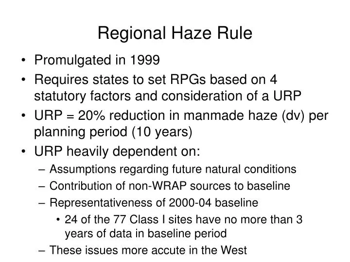
Regional Haze Rule. Promulgated in 1999 Requires states to set RPGs based on 4 statutory factors and consideration of a URP URP = 20% reduction in manmade haze (dv) per planning period (10 years) URP heavily dependent on: Assumptions regarding future natural conditions

E N D
Regional Haze Rule • Promulgated in 1999 • Requires states to set RPGs based on 4 statutory factors and consideration of a URP • URP = 20% reduction in manmade haze (dv) per planning period (10 years) • URP heavily dependent on: • Assumptions regarding future natural conditions • Contribution of non-WRAP sources to baseline • Representativeness of 2000-04 baseline • 24 of the 77 Class I sites have no more than 3 years of data in baseline period • These issues more accute in the West
Why A Species-Based Approach? • Species differ significantly from one another in their: • Contribution to visibility impairment • Spatial and seasonal distributions • Source types • Contribution from natrual and international sources • Emissions data quality • Atmospheric science quality • Tools available for assessment and projection
What Is A Potential Process? • For each site and species: • Estimate progress expected from Base Case + BART in 2018 • Determine any other LTSs which may be reasonable for that pollutant and recalculate 2018 species concentration • Add up improvements from all species into dv • This becomes the RPG for the 20% worst days • Explain why this is less than URP • Large international and natural contributions, large uncertainties in dust inventory preclude action, etc.
Determining Non-BART LTSs • Determine species glidepath and 2018 URP value • Estimate progress expected from Base Case + BART in 2018 • If progress is better than or equal to 2018 URP: • Check inventory for “important sources” which may be uncontrolled • If progress is worse than 2018 URP, but WRAP antho contribution declines by at least 20%: • Check inventory for important sources which may be uncontrolled
Determining Non-BART LTSs • If progress is worse than 2018 URP, and WRAP antho contribution declines by less than 20%: • Evaluate air quality & emission trends in more detail • Check inventory for important sources which may be uncontrolled or undercontrolled • Identify LTSs for these sources considering the 4 RPG factors and 7 LTS factors, where applicable • Either adopt these strategies, commit to adopting them post 2007, or commit to evaluating them further
“Important Sources” • Identified and qualitatively ranked based on some or all of the following: • Size, proximity, current/potential degree of control, feasibility of control, cost effectiveness, etc. • If point sources important, identify ~10 facilities • If area sources important, identify 3-5 categories • Identification of important sources should not be limitted by state boundaries
Determine URP for a species Is Base+BART projection better than URP? Is WRAP Anthro reduction > 20%? N N Evaluate emission & air quality trends more closely Y Y Are there any important uncontrolled or undercontrolled sources? Are there any important uncontrolled sources? Y Y Identify LTSs for these sources. Adopt, commit to adopt, or commit to further evaluation. N N Determine reductions at C1A. Repeat for other species. Add up all species reductions to get a RPG. Explain why it’s less than default URP but still reasonable. Note, if projection is better than URP and/or WRAP anthro reduction is >20%, the 4 RPG factors are inherently taken into account via BART.
Do SO4, NO3, OC, and EC meet their glidepaths? No, Yes, No, Yes. Then do the WRAP anthro contributions for SO4 and OC decline by 20%?
SO4 and NO3 Data • The following 6 slides describe and show the results of the CAMx-PSAT source apportionment model results for SO4 and NO3. • Results are used to determine the rank and significance of sources and to evaluate the percent change in their contribution to haze in the baseline and future years. They are not used to predict a specific amount / concentration of pollution.
SO4 and NO3 Apportionment • CAMx air quality model with PM Source Apportionment Technology (PSAT) • PSAT completed for 2 cases: • Plan 2002c • Base 2018b • Tracks sources of sulfate and nitrate • Tracking organic carbon too computationally intensive. However, data is available that delineates primary OC, from biogenic SOA, and anthropogenic SOA.
Eight Source Categories • Examples of PSAT “sources”: • MV_CO = mobile sources in Colorado • PT_CE = point sorces in CENRAP • BCON = transport from modeling domain boundaries (derived from GEOS-CHEM)
Status of Modeling • Plan 2002c just completed • Base 2018b completed end of August • Results currently available for daily and monthly averages • Results will be provided for 20% best and worst visibility days at each Class I area • See “Apportionment” link on TSS for results
Do WRAP anthropogenic SO4 contributions decline by 20%? Not quite (18%). Note: WRAP reductions would be significantly larger if 2001 were used as a base year because the first Centralia cut occurred in 2002. Also, OR_PT contribution will likely decline with BART, especially at the Boardman power plant.
Do WRAP anthropogenic NO3 contributions decline by 20%? Yes (39%). Again, note potential reductions from Boardman.
Carbon and Dust Apportionment • PSAT results for OC and EC not available due to computational resources. • No air quality modeling results available whatsoever for CM, and FS due to poor model peformance. • For these pollutants, an alternative technique developed by the WRAP could be used to evaluate sources and progress. • Weighted Emissions Potential (WEP)
Weighted Emissions Potential Method • Combine gridded emissions data with gridded backtrajectory residence times to determine sources with the most potential to affect a site. • Sources with the greatest potential will tend to be both upwind on the worst visibility days and have relatively large emissions. • 2002 and 2018 annual average emissions • 3-5 years of 20% worst days back trajectories • Discount sources based on distance from site • Ignore grid cells with very low residence times • Does not account for chemistry, dispersion, deposition • Method being finalized
Weighted Emissions Potential MethodPrototype example for Salt Creek, New Mexico Residence Times Weighted Emissions Potential = Emissions X
Do WRAP upwind weighted anthro OC emissions decline by 20%? No. They hardly change.
Do WRAP upwind weighted anthro VOC emissions decline by 20%? No. They hardly change because growth in point and area sources offsets mobile source reductions.
Do WRAP upwind weighted anthro EC emissions decline by 20%? Yes, 28% due to mobile source controls.
Do WRAP upwind weighted anthro CM emissions decline by 20%? No, they increase 32%.