Risk and Returns (Ch 12, 13) Returns Average Returns, Risk Premiums, Return Variability

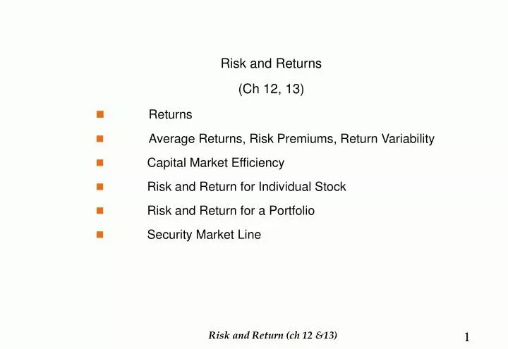
1. Risk and Returns (Ch 12, 13) • Returns • Average Returns, Risk Premiums, Return Variability • Capital Market Efficiency • Risk and Return for Individual Stock • Risk and Return for a Portfolio • Security Market Line 1 Risk and Return (ch 12 &13)

2. 1. Return in General -- Percentage Returns

3. Percentage Returns (Figure 12.2) (concluded) Dividends paid at Change in market end of period value over periodPercentage return = Beginning market value The first component is percentage of dividend income while the second component is capital gain +

4. A $1 Investment in Different Types of Portfolios: 1926-1998 (Fig. 12.4) Quickly go through figures for different types of companies (p360—p362)

6. Historical Dividend Yield on Common Stocks 10% 9 8 7 6 5 4 3 2 1

7. 2. Average Return, Risk Premium, and Return Variability • Average Returns– average of historical returns • see Table 12.1, and 12.2 (P365) • Risk Premium – the excess return required from an investment in a risky asset over that required from a risk-free investment • See Table 12.3 (next slide) • Variance and Standard Deviation of Returns (p367-368) When using historical data, variance is equal to: 1 _ [(R1 - R)2 + . . . [(RT - R)2] T - 1 _____

8. Average Annual Returns and Risk Premiums: 1926-1998 (Table 12.3) Investment Average Return Risk Premium Large-company stocks 13.2% 9.4% Small-company stocks 17.4 13.6 Long-term corporate bonds 6.1 2.3 Long-term government bonds 5.7 1.9 U.S. Treasury bills 3.8 0.0

9. Using Capital Market History (continued) • Risk premiums: First, we calculate risk premiums. The risk premium is the difference between a risky investment’s return and that of a riskless asset. Based on historical data: Investment Average Standard Risk return deviation premium Common stocks 13.2% 20.3% ____% Small stocks 17.4% 33.8% ____% LT Corporates 6.1% 8.6% ____% Long-term 5.7% 9.2% ____%Treasury bonds Treasury bills 3.8% 3.2% ____%

10. Frequency Distribution of Returns on Common Stocks, 1926-1998

11. We may Model this through Normal Distribution

12. 3. Market Efficiency • Efficient Capital Market • A market in which security prices reflect available information • Behavior in an efficient market • See the next slide – is it possible? • Dart versus Expert • Forms of Market Efficiency • Weak form – past information • Semistrong form– public information • Strong form – all information

13. Reaction of Stock Price to New Information in Efficient and Inefficient Markets Price ($) Overreaction andcorrection 220 180 140 100 Delayed reaction Efficient market reaction Days relativeto announcement day +4 +6 –4 –2 0 +2 +7 –8 –6 Efficient market reaction: The price instantaneously adjusts to and fully reflects new information; there is no tendency for subsequent increases and decreases.Delayed reaction:The price partially adjusts to the new information; 8 days elapse before the price completely reflects the new informationOverreaction:The price overadjusts to the new information; it “overshoots” the new price and subsequently corrects.

14. 4. Expected Return and Variance: Individual Stock • The quantification of risk and return is a crucial aspect of modern finance. It is not possible to make “good” (i.e., value-maximizing) financial decisions unless one understands the relationship between risk and return. • Rational investors like returns and dislike risk. • Consider the following proxies for return and risk: Expected return - weighted average of the distribution of possible returns in the future. Variance of returns - a measure of the dispersion of the distribution of possible returns in the future.

15. Example 1: Calculating the Expected Return and Variance – individual stock pi Ri Probability Return inState of Economy of state i state i +1% change in GNP .25 -5% +2% change in GNP .50 15% +3% change in GNP .25 35%

16. Example 1 – expected Returns i (pi Ri) i = 1 -1.25% i = 2 7.50% i = 3 8.75% Expected return = (-1.25 + 7.50 + 8.75) = 15%

17. Example 1 -- Variance i (Ri - R)2 pi (Ri - R)2 i=1 .04 .01 i=2 0 0 i=3 .04 .01 Var(R) = .02 What is the standard deviation? The standard deviation = (.02)1/2 = .1414 .

18. 5. Expected Returns and Variances -- Portfolio State of the Probability Return on Return oneconomy of state asset A asset B Boom 0.40 30% -5% Bust 0.60 -10% 25% 1.00 • A. Expected returns E(RA) = 0.40  (.30) + 0.60  (-.10) = .06 = 6% E(RB) = 0.40  (-.05) + 0.60  (.25) = .13 = 13% Example 2

19. Example 2 • B. Variances Var(RA) = 0.40  (.30 - .06)2 + 0.60  (-.10 - .06)2 = .0384 Var(RB) = 0.40  (-.05 - .13)2 + 0.60  (.25 - .13)2 = .0216 • C. Standard deviations SD(RA) = (.0384)1/2 = .196 = 19.6% SD(RB) = (.0216)1/2 = .147 = 14.7%

20. Example 2 • Portfolio weights: put 50% in Asset A and 50% in Asset B: State of the Probability Return Return Return oneconomy of state on A on B portfolio Boom 0.40 30% -5% 12.5% Bust 0.60 -10% 25% 7.5% 1.00

21. Example 2 • A. E(RP) = 0.40  (.125) + 0.60  (.075) = .095 = 9.5% • B. Var(RP) = 0.40  (.125 - .095)2 + 0.60  (.075 - .095)2 = .0006 • C. SD(RP) = (.0006)1/2 = .0245 = 2.45% • Note: E(RP) = .50  E(RA) + .50  E(RB) = 9.5% • BUT: Var (RP)  .50  Var(RA) + .50  Var(RB)

22. Example 2: with different weights • New portfolio weights: put 3/7 in A and 4/7 in B: State of the Probability Return Return Return oneconomy of state on A on B portfolio Boom 0.40 30% -5% 10% Bust 0.60 -10% 25% 10% 1.00 • A. E(RP) = 10% • B. SD(RP) = 0%

23. 6. Security Market Line • Key issues: • What are the components of the total return? • What are the different types of risk? • Expected and Unexpected Returns Total return = Expected return + Unexpected return R = E(R) + U • Announcements and News Announcement = Expected part + Surprise

24. Portfolio Diversification (Figure 13.1)

25. Beta Coefficients for Selected Companies (Table 13.8) Beta Company Coefficient American Electric Power .65 Exxon .80 IBM .95 Wal-Mart 1.15 General Motors 1.05 Harley-Davidson 1.20 Papa Johns 1.45 America Online 1.65 Source: From Value Line Investment Survey, May 8, 1998.

26. Example: Portfolio Beta Calculations Amount PortfolioStock Invested Weights Beta (1) (2) (3) (4) (3)  (4) Haskell Mfg. $ 6,000 50% 0.90 0.450 Cleaver, Inc. 4,000 33% 1.10 0.367 Rutherford Co. 2,000 17% 1.30 0.217 Portfolio $12,000 100% 1.034 Simple!!

27. Return, Risk, and Equilibrium • Key issues: • What is the relationship between risk and return? • What does security market equilibrium look like? The fundamental conclusion is that the ratio of the risk premium to beta is the same for every asset. In other words, the reward-to-risk ratio is constant and equal to E(Ri ) - Rf Reward/risk ratio = i 

28. Return, Risk, and Equilibrium (concluded) • Example: Asset A has an expected return of 12% and a beta of 1.40. Asset B has an expected return of 8% and a beta of 0.80. Are these assets valued correctly relative to each other if the risk-free rate is 5%? a. For A, (.12 - .05)/1.40 = ________ b. For B, (.08 - .05)/0.80 = ________ • What would the risk-free rate have to be for these assets to be correctly valued? (.12 - Rf)/1.40 = (.08 - Rf)/0.80 Rf = ________

29. The Capital Asset Pricing Model • The Capital Asset Pricing Model (CAPM) - an equilibrium model of the relationship between risk and return. What determines an asset’s expected return? • The risk-free rate - the pure time value of money • The market risk premium - the reward for bearing systematic risk • The beta coefficient - a measure of the amount of systematic risk present in a particular asset The CAPM: E(Ri ) = Rf+ [E(RM ) - Rf ] i 

30. The Security Market Line (SML) (Figure 13.4)