Baseflow Separation Techniques

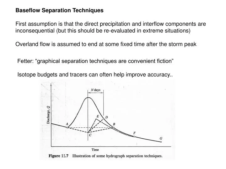
1. Baseflow Separation Techniques First assumption is that the direct precipitation and interflow components are inconsequential (but this should be re-evaluated in extreme situations) Overland flow is assumed to end at some fixed time after the storm peak Fetter: “graphical separation techniques are convenient fiction” Isotope budgets and tracers can often help improve accuracy..

2. Gaining and Losing streams Gaining (effluent) stream - baseflow entering stream - typical in humid regions - as you move down stream, more water in stream even though no tributaries exist Losing (influent) stream - water table lower than bottom of stream channel - water loss as you go down stream - rate of loss is a function of the depth of water and hydraulic conductivity of the underlying alluvium - In some cases (mountainous arid regions), you start with a gaining stream and move into a losing stream..

3. - During baseflow recession a stream may be gaining, but become a losing stream during floods

5. - ground-water pumping near a stream can drop the water table locally and cause a section of stream to be losing, while it is gaining up and downstream

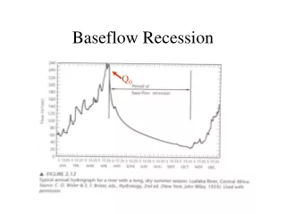
6. Baseflow Recession Understanding of baseflow recession is necessary before we can look at hydrograph separation - baseflow of a stream decreases during a dry period because as ground water flows into the stream the water table falls Baseflow recession equation is: where Q is the flow at some time t after recession has started Q0 is the flow at the start of the recession a is a recession constant for the basin t is the time since recession began e is base of natural logs -plotting Q vs t on semilog paper should yield a straight line (with t on the linear scale) - If more than one straight line apparent, there may be two groundwater sources - in most watersheds groundwater depletion characteristics are ~ stable since they closely match watershed geology..

9. Determining Baseflow Storage and Ground-water Recharge from Baseflow • Seasonal Recession Method • Assumes no dams or other regulation and minimal snowmelt • Need hydrographs from two or more consecutive years • using approximations derived from the baseflow recession equation we find: • Where: Vtp is the total potential volume of groundwater discharge (i.e. volume of water discharged during complete recession) • Qo is baseflow at the start of recession • t1 is the time for baseflow to go from q0 to 0.1q0..

10. - If the amount of baseflow in the reservoir is calculated at the end of a recession and then the beginning of the next recession the amount of recharge can be obtained by the difference - hence the amount of baseflow remaining at any time after baseflow recession begins is: - the above assumes no consumptive use during the time period of interest..

11. 10,000 1000 cfs 100 10 0 • Recession Curve displacement method • More suited to areas without strong seasonal dry periods • t1 is the time for recession to cover one log cycle • t1 needs to exceed D from equation • Where D = days between storm peak and • end of overland flow • A = basin area (mi2) • tc is a critical time which is 0.2144t1 Recharge is calculated as: T1 = 45 days for this chart

12. Rainfall-Runoff Relationships • - basic goal is to predict amount of runoff that will occur from a given storm • - need to design structures and neighborhoods based on peak discharges • Rational Equation is simplest • if it rains long enough, peak Q from basin will be the average rate of rain times • the basin area (adjust by a coefficient to account for infiltration) • time of precip has to exceed time of concentration for rational equation to apply • - time of concentration is time necessary for water to flow from the most distant part of watershed to point of discharge • - conceptually time of concentration is the average velocity of the longest stream channel times the length of the channel, plus time for overland flow to reach the channel..

13. - rational equation assumes constant rainfall and infiltration rate - best used for small (200 acres or less) watersheds Q is peak runoff rate I is average rainfall intensity A is the drainage area C is a runoff coefficient (gotten from a table) Lower range of C is used for low intensity storms Higher range for high intensity storms..

14. Duration Curves - often want to know how often a stream flows at a lesser or greater discharge than some value - duration curves usually daily or annual flow Steps are: 1. Rank flow records (m) starting with 1 for highest flow and n for lowest over the period of interest (if two are equal, they each get their own rank...no ties) 2. The probability (P) that a given flow will be equaled or exceeded is given by: 3. If comparing multiple rivers reduce Q to discharge per unit area of basin (e.g. m3/s/km2 4. On probability paper (or in spreadsheet) Plot Q as Y-axis and P as x-axis - distribution of runoff is caused by geology of drainage basin - steeper curves have thinner soils, lower hydraulic conductivity, less overall baseflow..

15. Connect the stream with the Basin character: 2. Thick sand deposits 3. Glacial till with silt and clay

16. Unit Hydrographs • - a unit hydrograph is the characteristic response of a given watershed to a unit volume (depth) of effective water input applied at a constant rate • - used to forecast response of a watershed to a given input of water • - hydrograph of direct runoff (excludes baseflow) • To develop unit hydrograph (1") • 1. Collect as much streamflow and precip data as possible • Best storms are: a) individual • b) uniform temporal and spatial distribution • c) rainfall duration should be ~10-30% of basin lag time • d) direct runoff should range from 0.5 to 1.75 inches • 2. For each storm, separate quickflow and baseflow • 3. Calculate depth of direct runoff (quickflow) per hour (from beginning of quickflow)..

17. 4. Multiply each original hydrograph by 1 over value in obtained in 3. 5. 6. Plot several unit hydrographs for similar duration rains in this way 7. Construct composite unit hydrograph: take peak as average in both x and y, and adjust until area under curve is 1" of runoff With say a 2.5 hour unit hydrograph can then take a forecast precipitation of say 2" and just double the height of your 1" inch unit hydrograph to come up with prediction of stream response to forecast storm. Urban Hydrology - urbanization generally increases total quickflow for a given rainfall - faster time to peak (lower time of concentration) and higher peak - lower rates of ground water recharge in area of urban centers - serious in areas where ground-water is big portion of supply..