Download
1 / 20
200 likes | 353 Views
Hierarchical packet classification using a Bloom filter and rule-priority tries. Source : Computer Communications Authors : A. G. Alagu Priya 、 Hyesook Lim Publisher : Butterworth-Heinemann Newton, MA, USA Presenter : JHAO-YAN JIAN Date : 2010/9/15. Outline. Introduction ALBF RPT

E N D
Hierarchical packet classification using a Bloom filter and rule-priority tries Source : Computer Communications Authors : A. G. Alagu Priya、Hyesook Lim Publisher : Butterworth-Heinemann Newton, MA, USA Presenter : JHAO-YAN JIAN Date : 2010/9/15
Outline Introduction ALBF RPT Performance Evaluation
Introduction • TCAM based solutions are the one which offers consistently a high performance independent of the characteristics of the rule set. • However, the cost and high power consumption of TCAM made to explore some other algorithmic solutions • fast algorithm based on Bloom filters • the Bloom filter is used to avoid lookup in some subsets which contain no matching. • It can be implemented with on-chip memory or a fast cache.
Bloom filter(1/2) • Bloom filter is a space-efficient probabilistic data structure that is used to test whether an element is a member of a set. • IP address lookup algorithms using Bloom filter and assign each distinct prefix length a Bloom filter. • To design a Bloom filter which can accommodate various lengths of prefixes in it.
Bloom filter(2/2) S. Dharmapurikar, P. Krishnamurthy, D. Taylor, Longest prefix matching using Bloom filters, in: Proc. of ACM SIGCOMM, August 2003, pp. 201–212.
Hierarchical approach • Algorithm based on a hierarchical approach. • First stage : ALBF(all-length Bloom filter) • Accommodates different length of prefixes in a single Bloom filter • ALBF is constructed based on source prefixes • Second stage : RPT(rule-priority trie) • RPT is constructed based on destination prefixes
ALBF(1/2) Prefix CRC code Hash indices 010* 111000 14, 8 101* 101101 11, 13 1* 110001 12, 1 1101* 100011 8, 3 110100* 111000 14, 8 111* 010101 5, 5 b0(t+1) = input XOR b5(t) b1(t+1) = input XOR b0(t) b2(t+1) = b1(t) b3(t+1) = b2(t) b4(t+1) = b3(t) b5(t+1) = input XOR b4(t) CRC-6 generator • Hash generator • Any number of hash indices can be easily obtained from the generated CRC code by selecting several different combinations of bits • First 4 bits & Last 4 bits
ALBF(2/2) ALBF programmed for distinct source prefixes • There are two factors affecting the performance of a Bloom filter: the size of the Bloom filter and the number of hash indices. • To determine the size m of the ALBF : • n : the number of non-wild source prefixes • 2z : the size of the Bloom filter m • 2(z-1)<(n×I)<=2z, whereI is a multiplication factor andz>0. • In selecting two hash indices from a CRC code, we consistently selected the first z bits and the last z bits for two hash indices, k1 and k2. The bit-locations k1 and k2 in the ALBF are set as 1.
RPT(1/2) proposed rule-priority trie (RPT) is based on the priority trie, but relocating the highest-priority rule instead of the longest-prefix rule. The relocated rule is termed as a priority rule, and a rule stored in its own level is termed as an ordinary rule. nodes in the RPT will have information about entire rule fields. If the destination prefix reaches its own position, in which the node position corresponds to the destination prefix, even if the node had a higher-priority rule, the rule has to be replaced.
RPT(2/2) Rule Prefix R1 010* R2 101* R3 * R4 1* R1 R1 R2 R3 R2 R1 R3 R4 R1 R2 If we assume that rules are sorted first in the order of decreasing priority, the pushing is not frequently occurred. Search in the proposed algorithm is finished either at a match with a priority rule or at a leaf while it is always finished at a leaf in other trie-based algorithms.
Packet classification approach(1/3) Packet classification approach follows the observation from real databases that any packet matches only a small number of distinct source-destination prefix pairs. The port range specifications stay as ranges without the blowups associated with range translation. Since the rules with source prefix as wild-card (*) cannot be programmed in the ALBF, a separate RPT is created for those rules, and it is termed as RPT-wild. After constructing every RPT, we denote the threshold value for each RPT, where the threshold value of a RPT is equal to the highest-priority rule included in that RPT.
Packet classification approach(2/3) RuleSrc prefixDest prefix Src port Dest portProtocol R0 010* 10* 0,65535 25,25 6 R1 101* 001* 53,53 443,443 4 R2 * 10* 53,53 1024,65535 17 R3 * 01* 53,53 443,443 4 R4 1* 1* 53,53 25,25 4 R5 1101* 001* 0,65535 2788,2788 17 R6 110100* 11* 53,53 5632,5632 6 R7 * 11* 53,53 25,25 6 R8 111* 01* 67,67 5632,5632 17 R9 010* 10* 0,65535 0,102 6 R10 111* 1* 67,67 25,25 4 R11 1101* 001* 53,53 2788,2788 4 R12 111* * 1024,65535 5632,5632 4
Packet classification approach(3/3) • Searching : • The search procedure is repeated for the sub-string of the source address with the next smaller distinct length, and if the Bloom filter gives a positive result, the search will be continued in the corresponding RPT-k1. • Once a RPT is accessed, then that trie will be disabled. • If the already found match has a higher priority than the threshold, that trie is not necessarily searched. • The RPT-wild is accessed only if its threshold value has a higher priority than the already found match.
Incremental update • Insert: • If the new rule has a source prefix length which is different from the lengths of already stored prefixes, then the distinct lengths of prefixes stored in ALBF are updated. • The rule is inserted into the corresponding RPT. • Delete • the rule can be removed from the RPT and that empty location can be filled with the next priority rule in that sub-trie. • the representation of source prefix of that rule cannot be deleted from the ALBF, because the corresponding bit-locations of k1 and k2 of that prefixes may also represent some other prefixes. • The problem can be solved using a counting Bloom filter.
Simulation Results(1/6) CRC-6 generator Three different types of rule sets, ACL, FW, and IPC, are created with sizes of about 1000 and 5000 rules, each. a 32-bit CRC generator to provide hash indices for all-length Bloom filter (ALBF)
Simulation Results(3/6) Proposed : multiplication factor I is set as ‘1’. Hierarchical trie (H-trie) set-pruning trie Hierarchical binary search tree (HBST) algorithm is the same as the H-trie except that HBST replaces the trie structure in H-trie with the tree structure which does not include empty internal nodes. Area-based quad-trie (AQT) recursively partitions a 2-dimensional plane composed of source and destination prefixes, and each partitioned area is mapped to a quad-trie node. Priority-based quad-trie (PQT) algorithm is based on the AQT algorithm, but empty nodes in the AQT are completely avoided. Binary search on prefix length (BSL) Bit-vector (BV) Hicut & Hypercut : high binth and cuts in each dimension are set to 4.
Simulation Results(4/6) Average number of memory accesses for 1K rule sets Worst case number of memory accesses for 1K rule sets
Simulation Results(5/6) Average number of memory accesses for 5K rule sets Worst case number of memory accesses for 5K rule sets
Simulation Results(6/6) Memory requirements for 1K rule sets (Kbytes) Memory requirements for 5K rule sets (Kbytes)