Download
1 / 83
860 likes | 1.14k Views
Maa-57.2040 Kaukokartoituksen yleiskurssi General Remote Sensing Image restoration. Autumn 2007 Markus Törmä Markus.Torma@tkk.fi. Digital image processing. Image is manipulated using computer Image mathematical operation new image Application areas: Image restoration

E N D
Maa-57.2040 Kaukokartoituksen yleiskurssiGeneral Remote SensingImage restoration Autumn 2007 Markus Törmä Markus.Torma@tkk.fi
Digital image processing • Image is manipulated using computer • Image mathematical operation new image • Application areas: • Image restoration • Image enhancement • Image interpretation / classification
Image restoration • Errors due to imaging process are removed • Geometric errors • position of image pixel is not correct one when compared to ground • Radiometric errors • measured radiation do not correspond radiation leaving ground • Aim is to form faultless image of scene
Image enhancement • Image is made better suitable for interpretation • Different objects will be seen better manipulation of image contrast and colors • Different features (e.g. linear features) will be seen better e.g. filtering methods • Multispectral images: combination of image channels to compress and enhance imformation • ratio images • image transformations • Necessary information is emphasized, unnecessary removed
Digital image processing • Analog signal: • phenomena is described of measured continuosly according to time or space • Digital signal: • analog signal is sampled with some interval • 2-dimensional digital signal digital image
Digital image processing Image function f(x,y): • Function according to spatial coordinates x and y • Value of function in position (x,y) corresponds to brightness of image in corresponding position
Digital image processing • Digital image consists of individual picture elements, pixels, which form discere lattice in spatial domain (x,y) • Digital image can also be presented using SIN-waves with different frequencies and amplitudes • called frequence domain (u,v) • Fourier transform is used to determine frequencies • Manipulation of digital image: • Image domain: pixel values are modified directly at iomage using some algorithm • Spatial domain: frequencies and amplitudes of SIN-waves are modified
Sources of error Movement opf imaging platform • Changes in height or speed • Attitude of satellite Image provider should correct Instrument • Scanning or measurement principle • Failures of sensors • Production methods or accuracy of instrument Calibration of instrument
Sources of error Atmosphere • Attenuation of radiation and decrease of contrast • Image is blurred Difficult to correct Object • Roundness of Earth • Rotation of Earth • Topography It is possible to cerrect these quite well
Geometric correction • Position of image pixel is not correct when compared to ground • Errors due to instrument, movement of imaging platform and object are removed • Known errors in geometry: • Earth cirvature and rotation • Topography • Imaging geometry • Rectification to map projection • Geometric transformation • Interpolation of pixel digital numbers
Geometric correction • Geometric correction is made • automatically using orbital parameters or • manually using ground control points • Alternatives • orbital parameters • ground control points • orthocorrection • Most accurate results by combining all
Raw image data • It can be difficult to recognize ground features from raw image data, because they are not necessarily similar than in nature
Geometric correction using orbital parameters • Information about • position of satellite (XYZ) • attitude () • Correction can be low quality due to poor orbital information • Knowledge about scanning geometry, movement of object and topography (DEM) will increase accuracy
Geometric correction • Accuracy of correction depends on quality of used information • Some examples about accuracy using orbital parameters: • NOAA AVHRR: 5 km - 1.5 km • Spot 1-4: 350 m • Spot 5: 50 m • Ground control points: accuracy should be better than 1 pixel • depends also mathematical model and topographic variations • Orthocorrection most accurate
Geometric correction Manual correction: • Ground control points (GCPs): • image coordinates are measured from image • map coordinates from map or georeferenced image
Geometric correction • GCPs are known and well distinguished ground features • crossroads, buildings, small lakes, small islands, features in waterline • More GCPs is better • When transformation between image coordinate system and map coordinate system is defined using polynomials, minimum number of points: • 1st degree polynomial: 3 points • 2nd degree: polynomial: 6 points
Example • Erdas Imagine • Old Landsat TM-image is georeferenced to same map coordinate system than Landsat ETM-image
Example • 2nd degree polynomial • 15 GCPs
Automatic correction • Software searches corresponding points from image to be georeferenced and image in map coordinate system • This can be based on • correlation between subimages • recognizable features (linear like roads or lakes) • These points are used as GCPs • Software produces many (e.g. 200-300 points for Landsat ETM-image) • user has to select which can be used • Automatization is needed when there are many images and/or it has to be made daily
Topographic error • Property of imaging system using central projection • Image of object is in incorrect place due to height variations
Orthocorrection • Topographic error is removed by changing the perspective of image from central projection to orthogonal projection • DEM is needed
Interpolation of digital numbers • Digital numbers for pixels of corrected image must be interpolated from uncorrected image • Seldomly number from uncorrected image can be used directly • Methods • nearest neighbor interpolation • bilinear interpolation • cubic convolution interpolation
Nearest neighbor interpolation • Take value of closest pixel from uncorrected image • Easy to compute • Values do not change • Result can be inaccurate korjattu kuva alkuperäinen kuva
Nearest neighbor interpolation • Values of some pixels are chosen more than once, some not at all • ”Piecewise” image • Linear features can disappear korjattu kuva alkuperäinen kuva
Bilinear interpolation • 4 closest pixels from uncorrected image are used • Average weighted by distance • Changes digital numbers • corresponds to average filtering korjattu kuva alkuperäinen kuva
Cubic convolution • 16 (4x4) closest pixels from uncorrected image are used • Smaller interpolation error than NN or BL-interpolation korjattu kuva alkuperäinen kuva
Alkuperäinen kuva lähin naapuri bilineaarinen kuutio
Image formation • Scene f(x) • Acquired image g(x) • Scene f(x) is corrupted by atmosphere and instrument in imaging process • They act like filters h(x)
Image formation • Image acquisition can be modelled with image degradation model: f(x) * h(x) + n(x) = g(x) g(x): acquired image h(x): filter corresponding to averaging effects due to atmosphere and instrument n(x): random errors due to instrument and data transmission f(x): scene
Inverse filtering • Errorness image of scene f(x) should be acquired by making inverse process to known image g(x) • Image degradation model in frequency domain: G(u)=F(u)H(u)+N(u) • Ideal inverse filtering Fe(u) = G(u)/H(u) - N(u)/H(u) • In practice difficult to solve • zeros in H(u) • effect of N(u) increases • Usually radiometric correction is divided to different phases which are corrected individually
Radiometric correction • In order that measurements taken with • different instruments • differents dates are comparable • Aim: radiance or reflectance • Radiance (W/m2/sr): • physical term which describes intensity of radiation leaving ground to some direction • Reflectance: • Radiance / incoming irradiance
Instrument calibration • Instruments are calibrated before satellite launch • measurements of known targets • instrument response is followed by measuring calibration targets in instrument or stable targets on ground • Each channel have calibration coefficients GAIN and OFFSET • these can vary within time • response decreases, so same target looks more dark
Instrument gain • Pixel digital number is multiplied with gain radiance = Dn * Gain • Gain = Lmax – Lmin / 255 • Lmax: largest radiance which can be measured by instrument • Lmin: smallest radiance which can be measured by instrument
Instrument offset • Background noide detected by instrument • Measurement, when instrument do not receive any radiation = Lmin
Radiometric correction • Equation: R = (Lmax-Lmin)/255*DN + Lmin OR R=Gain*DN + offset
Other corrections • Sun zenith angle: DN’=DN / SIN(sunq) • Ground is illuminated differently when Sun zenith angle changes • seasonal differences
Other corrections : • Distance between Sun and Earth • This distance varies according to seasons • Irradiance incoming to ground is when taking sun zenith angle into account:
Atmospheric correction • Absorption and scattering • Decrease of diffuse skylight • due to atmospheric scattering • largest at smaller waveleghts (blue), decreases as wavelenght increases • dampens image contrast
Atmospheric correction • REF: reflectance of pixel • Lsat: radiance measured by instrument • Lhaze: radiance due to atmospheric scattering (diffuse skylight) • TAUv: atmospheric transmittance from ground to instrument • E0: Sun spectral irradiance outside atmosphere, including effect of distance between Sun and Earth: E0 = E / d2, where E is Sun spectral irradiance outside atmosphere and d is distance between Sun and Earth in Astronomical Units • sz: Sun zenith angle • TAUz: atmospheric transmittance from Sun to ground • Edown: maanpinnalle tullut ilmakehän sironnan vaikutus
Atmospheric correction Apparent reflectance model • Removes effects of changing Sun-Earth distance and Sun zenith angle • changing imaging geometry • Does not remove atmospheric effects: absorption or scattering • Following parameters for correction model: TAUz: 1.0, TAUv: 1.0, Edown: 0.0, Lhaze: 0.0
Atmospheric correction DARK-OBJECT-SUBTRACTION • It is supposed that there are areas in image that are on shadow, so that all radiation coming to instrument from these areas is due to diffuse skylight • Following parameters for correction model : TAUz: 1.0 TAUv: 1.0 Edown: 0.0 Lhaze: measure radiance from target which is in shadow (like shadow of cloud) or does not reflect radiation (water in infrared)
Atmospheric correction CHAVEZ • Modified DOS • Atmospheric transmittances are approximated by angles of imaging geometry • Following parameters for correction model : TAUz: cos(sz) TAUv: 1.0 or cos(incidence angle) Edown: 0.0 Lhaze: measure radiance from target which is in shadow (like shadow of cloud) or does not reflect radiation (water in infrared)
Atmospheric correction • More theoretic methods try to model how radiation travels in atmosphere • Aim is to model • atmospheric transmittance and absorption • scattering due to gases • reflectances due to atmosphere, not ground • Difficult, requires lot of computing and precise knowledge about the state of atmosphere
VTT atmospheric correction • SMAC: Simplified Method of Atmospheric Correction • Removes Rayleigh scattering, absorption due to atmospheric gases, imaging geometry (sun anlges and distance) • Digital number reflectance • Needed calibration coefficients of instrument sun zenith and azimuth angles amount of water vapour ozone atmospheric optical depth
VTT atmospheric correction • Original Landsat ETM-images • Atmospheric optical Depth can be estimated from image if there are suitable channels • ETM7/ETM3 ratio should be about 0.4 for olf coniferous forests
VTT atmospheric correction • Corrected Landsat ETM-mosaic • Eastern Finland • 7 images • RGB: 321
VTT atmospheric correction Landsat ETM-mosaic of Northern Finland consists of 9 images
Dehazing image • Based on Tasselled Cap-transformation • TC4 image sensiive to atmospheric effects • Landsat-5 TM-image: TC4 = 0.8461*TM1 - 0.7031*TM2 - 0.4640*TM3 - 0.0032*TM4 - 0.0492*TM5 - 0.0119*TM7 + 0.7879 • Image channel is corrected by subtracting TC4 from it TMcx = TMx - (TC4 - TC40)*Ax TMcx: Corrected digital number of channel x TMx: Original digital number of channel x TC40: Value of haze-free pixel in TC4 Ax: Correction factor determined from image
Dehazing image • Original and corrected TM1