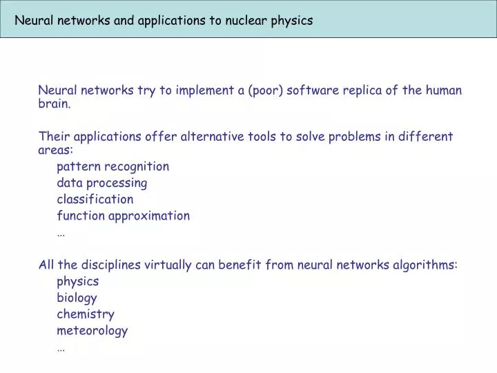
Neural networks and applications to nuclear physics

1. Neural networks and applications to nuclear physics Neural networks try to implement a (poor) software replica of the human brain. Their applications offer alternative tools to solve problems in different areas: pattern recognition data processing classification function approximation … All the disciplines virtually can benefit from neural networks algorithms: physics biology chemistry meteorology …

2. Traditional approaches vs. neural networks A conventional approach to a problem is based on a set of programmed instructions. In the neural network approach the solution is found learning from a set of examples. This is typical of the human brain, which employs the past experience to understand how to solve a similar problem, thus adapting itself as it gain additional experience. A traditional algorithm may be seen as a computer program with a fixed list of instructions, while an artificial neural network may be represented by instructions which change as additional data are known.

3. Traditional approaches vs. neural networks To implement this, an artificial neural network can be regarded as a non-linear mathematical function which transforms a set of input variables to a set of output variables, with parameters (weights) which are determined by looking to a set of input-output examples (learning or training phase). The learning phase may be also very long, but once the weigths are fixed, new cases are treated very rapidly. The important point is that no a priori exact relation must exist between inputs and outputs, which makes neural networks interesting tools when the problem has no explicit theoretical basis.

4. Traditional approaches vs. neural networks/2 A critical point is the need to provide the network with a realistic set of good examples in the learning phase, which is not so simple. Moreover, if the network is required to analyze examples which are too different from those learned in the first phse, its behaviour is not so good (as for the human brain!) Basically, neural networks are a good solution when: • It is possible to find a good set of training data • The problem has no first-principle theoretical model • New data must be processed in a fast way, after a long training phase • Noise on the data (fluctuations or variations) must not influence too much the results

5. Biological neural networks The human brain: the most complex structure known: 1011 neurons Two biological neurons Dendrites act as inputs When a neuron reaches the threshold, it gives an output through the axon. Interaction between neurons takes place at junctions, called synapsis. Actually, each neuron has connections to many thousands other neurons, so the total number of synapses are in the order of 1014.

6. Biological neural networks/2 Each neuron works on a time scale relatively slow (1 ms). However, this is a massive parallel system, so in a very short time, an impressive number of operations are done. The resulting speed is then larger than any existing computer. The large number of connections results in a fault-tolerant system (redundancy). Even if many neurons disappear each day, most of these connections are replicated and no significant difference in the overall performance is observed. On the contrary, even a single electrical connection in a PC makes the entire PC not working!

7. Biological neural networks/3 Most neurons produce a 0/1 output. When they “fire”, they send an output through the axon and the synapse to another neuron. Each synapse has an associated weight (strength). Each neuron then collects all the inputs coming from linked neurons, and computes a weighted sum of all inputs. A key property if the ability to modify the strengths of these synapses, i.e. the weights.

8. Artificial neural networks/1 Simple mathematical model of an artificial neuron (Mc Culloch-Pitts, 1943) It may be regarded as a non-linear function which transforms a set of inputs xi into the output z. Each input is multiplied by a weight wi (positive or negative) and then summed to the other inputs to produce a. A non-linear function g(a) produces the output z.

9. Artificial neural networks/2 Typical activation functions g(a) • Linear • Threshold • Threshold linear • Sigmoidal Original Mc Culloch-Pitts: (b) Most used today: (d)

10. Developments of neural network algorithms Origin: Mc Cullogh & Pitts, 1943 Late 1950’s: development of first hardware for neural computation (perceptron) Weights adjusted by means of potentiometers Capability to recognize patterns (characters, shapes,..) Years 60’s: a lot of developments and applications with software tools, often without solid foundations End of 60’s: Decrease of interest, since difficult problems could not be solved contrary to what expected From 1980’s: Renewed interest, due to improvements in learning methods (error backpropagation) and availability of powerful computers 1990’s: Consolidation of theoretical foundations, explosion of applications in several fields

11. Neural network architectures Two main architectures are used for neural networks Multilayer perceptron (MLP): the most widely diffused architecture for most of the present applications Radial basis function (RBF):

12. The multilayer perceptron A single layer architecture. Each line is a weight A multilayer structure: between inputs and outputs, one or more layers of hidden neurons

13. The learning phase The learning phase is accomplished by minimizing an error function to a set of training data, to extract the weights. This error function may be considered as a hyper-surface in the weight space, so the problem of training the network corresponds to a minimization problem in several variables. For a single-layer network and linear activation functions, the error function is quadratic and the problem has analytical solutions. For multilayer networks, the error function is a highly non-linear function of the weights parameters, and the search for the minimum is done through iterative methods. Several methods may be chosen by the user to carry out this phase Example of the error function E in the weight spaces (only 2 parameters)

14. The testing phase Once trained the network by a set of data, the question is: how good is the network to handle new data? Problem: If the netwok is trained with data with some “noise” and learns about the noise, it will give poor performance on data which do not exhibit such noise… Analogy with polynomial fitting Bad fit Good fit “Too good” fit

15. The testing phase Quality of the fit as a function of the polynomial order: On the training data the error goes to 0 when the curve passes through all the points. However, on new data the error reaches its minimum for n=3

16. The testing phase By analogy, if we increase the number of neurons in the hidden layer, the error on training always decreases, but on test data it reaches a minimum around the optimal value. In practical applications, to optimize the number of hidden units, one can divide the overall set of data in two sets, one for training, the other for testing the network. The best network is that which minimizes the error on the test data set.

17. The testing phase Example from a real application

18. Summarizing the process (1) Select a value for the number of hidden units in the network, and initialize the network weights using random numbers. (2) Minimize the error defined with respect to the training set data using one of the standard optimization algorithms such as conjugate gradients. The derivatives of the error function are obtained using the backpropagation algorithm as described in Sec. III. (3) Repeat the training process a number of times using different random initializations for the network weights. This represents an attempt to find good minima in the error function. The network having the smallest value of residual error is selected. (4) Test the trained network by evaluating the error function using the test set data. (5) Repeat the training and testing procedure for networks having different numbers of hidden units and select the network having smallest test error.

19. Typical examples in nuclear and particle physics A few examples to be discussed: Pattern recognition for particle tracks Selection of events by centrality Particle identification by energy loss Short-lived resonance decays Reconstruction of the impact point in a calorimeter On-line triggers

20. Track recognition A set of hits in a complex detector. Which points belong to the same track?

21. Track recognition

22. Track recognition

23. Classification of nuclear collisions by centrality Traditional methods to classify nuclear collisions into central, semicentral and peripheral collisions usually employ one or more global variables, which depend on the collisions centrality. Usually the use of a single variable fails. A neural network technique may be applied to such class of problems - Train the network on simulated events filtered by the detector limitations • Apply the network to experimental data

24. Classification of nuclear collisions by centrality Example: Analysis of Au+Au collision events at 600 A MeV (David & Aichelin, 1995) Simulated events: Au + Au collisions with bmin=0, bmax=14 fm by QMD model Normalized impact parameter b*= b/bmax (0 – 1) Preliminary analysis with traditional methods based on a single global variable Global variables tested: Total multiplicity of protons (MULT) Largest fragment observed in the collision (AMAX) Energy ratio in c.m. system (ERAT) Method: Evaluate in small bins of b (0.05) mean and variance of these variables Approximate the mean value –b dependence by a fit with a spline function

25. Classification of nuclear collisions by centrality Results: For central collisions (b< 3.5 fm): MULT and AMAX are nearly constant (no use) ERAT shows a dependence on b In peripheral collisions AMAX approaches a constant value MULT and ERAT show a dependence on b To evaluate the precision of the method, the fit function is inverted and the estimated impact parameter is compared with the “true” impact parameter by the standard deviation C:

26. Classification of nuclear collisions by centrality Comment: No single variable is able to select very well central collisions For instance, ERAT gives large fluctuations on central events

27. Classification of nuclear collisions by centrality Use of a neural network with the following architecture 3 input neurons 5 hidden neurons 1 output neuron Input neurons: 3 of the following variables: AMAX MULT ERAT IMF (Multiplicity of intermediate fragments) FLOW DIR …

28. Classification of nuclear collisions by centrality Quality of the result estimated by the standard deviation The value of the standard deviation as a function of the number of iterations

29. Classification of nuclear collisions by centrality Summary of results A factor of 3 better than ERAT only

30. Classification of nuclear collisions by centrality Summary of results

31. Particle identification by the ΔE-E measurement Identification of charged particles may be achieved by the combined information of energy loss ΔE and residual energy E in a telescope detector. Identifying different particles in many detectors require quite often a long manual process through two-dimensional cuts

32. Particle identification by the ΔE-E measurement Example: Si (300 micron) – CsI (6 cm) telescope (TRASMA detector @LNS) Ca+Ca @ 25 A MeV

33. Particle identification by the ΔE-E measurement A neural network may be implemented to reconstruct the energy E and the atomic number Z of the detected particle (Iacono Manno & Tudisco, 2000) Different network architectures tested Training on a set of 340 events and testing on 250 events

34. Particle identification by the ΔE-E measurement Results Difference between “true” and reconstructed values

35. Particle identification by the ΔE-E measurement Selection of particles according to their atomic number

36. Identification of the K*(892) short-lived resonance Topology of the K*(892) decay

37. Identification of the K*(892) short-lived resonance Traditional analysis based on multidimensional cuts Firstly, select K0s candidates, Then apply additional cuts to the associate pion tracks, and build invariant mass spectra

38. Identification of the K*(892) short-lived resonance Network topology 16:16:1 Implementing all the variables in a unique network for reconstruction of resonance Several architectures tested with similar results

39. Identification of the K*(892) short-lived resonance Network output result Cut at 0.3

40. Identification of the K*(892) short-lived resonance Invariant mass spectrum, after cutting on the neural network output at 0.3

41. Identification of the K*(892) short-lived resonance Purity vs efficiency Performance of the network, compared to traditional topological cuts

42. Neural networks for time series analysis: an application to weather forecast Time series are collections of data which result from observations with equal time intervals between them. Applications of time series are frequent in any field of science or economy. Examples: Environmental observations (pressure, temperature, humidity, …) Cosmic ray flux, solar flux,… Economical parameters: stock index, share quotas,.. Analysis of time series carried out for: • Understand the overall trend and patterns, periodicity,.. • Predict the beaviour of the series in the near future • Study autocorrelation or cross correlations • …

43. Neural networks for time series analysis: an application to weather forecast An example of a pressure time series along a period of about 2 weeks. Known 12 and 24 hours periodicity observed, superimposed to aperiodic variations, due to weather

44. Neural networks for time series analysis: an application to weather forecast Several forecast model exist to predict the atmospheric weather. In principle a simple neural network can be trained on a series of past values, to produce an output value (values at the next steps) Input neurons: Values of the quantity Xi (i= 0, -1, -2, -3,…) Output Values of the quantity Xi (i=+1,+2,…) Training phase: to be carried out on available observations Evaluation of the goodness of the method: Comparison between predicted and really observed values

45. Neural networks for time series analysis: an application to weather forecast Network topologies implemented: Input neurons: Values of the barometric pressure in the preceding 3-14 days Hidden layers: from 0 to 2 layers Final choice: 14-14-1 topology Normalized values of the pressure (970 mbar is the minimum, 80 mbar the range) Training on 1500 days (4.5 years) Testing on 500 days (1.5 years)

46. Neural networks for time series analysis: an application to weather forecast Results: distribution of the differences between predicted and really observed values of the atmospheric pressure over 1.5 years) The RMS (5.232) gives an idea of the forecast performance

47. Neural networks for time series analysis: an application to weather forecast In this case the method is not so good, although slightly better than others. For instance, comparison to ARIMA method (AutoRegressive Integrated Moving Average) RMS =5.664 instead of 5.232

48. Neural networks for time series analysis: an application to weather forecast Comparison to naive prediction: assume that the pressure tomorrow will be the same as today! Correlation between pressure values in consecutive days (nearly good correlation) …and between the pressure values 7days apart (the correlation is lost)

49. Neural networks for time series analysis: an application to weather forecast Comparison to naive prediction: assume that the pressure tomorrow will be the same as today! The RMS is 6.195, not so bad…

50. Neural networks for stand-alone tracking in the ALICE ITS Track finding and fitting in ALICE is usually done through a combination of the information provided by the ITS (6-layers of silicon detectors) and TPC (up to 160 space points). The method employed is the Kalman Filter algorithm. Perfomance of the method are evaluated by the tracking efficiency and momentum resolution. A study was carried out to implement a stand-alone ITS tracking (when the information from the TPC is not available) with a neural network.