Download
1 / 13
130 likes | 261 Views
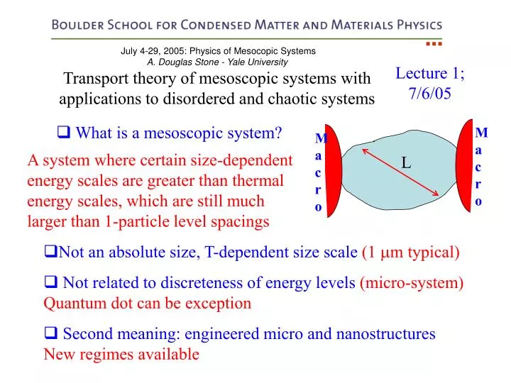
Macro. Macro. L. July 4-29, 2005: Physics of Mesocopic Systems A. Douglas Stone - Yale University Transport theory of mesoscopic systems with applications to disordered and chaotic systems. Lecture 1; 7/6/05. What is a mesoscopic system?.

E N D
Macro Macro L July 4-29, 2005: Physics of Mesocopic Systems A. Douglas Stone - Yale University Transport theory of mesoscopic systems with applications to disordered and chaotic systems Lecture 1; 7/6/05 • What is a mesoscopic system? A system where certain size-dependent energy scales are greater than thermal energy scales, which are still much larger than 1-particle level spacings • Not an absolute size, T-dependent size scale (1 m typical) • Not related to discreteness of energy levels (micro-system)Quantum dot can be exception • Second meaning: engineered micro and nanostructuresNew regimes available
L • Thermal energy/time scales?kBT, h/(kBT) Transport energy/time scales: Ballistic limit: • erg = L/vf(Eerg = hvf/L = 1d level spacing >> ) • esc = L/(vf p1) (p1 = escape prob/bounce)open system: p1 > 1/(kfL)d-1 ≈ Nc => Eesc ≥ Diffusive limit: l < L • erg = L2/D => ETh = hD/L2(Thouless energy) • esc = L2/Dp1 => Eesc = p1ETh(often assume p1 ≈ 1, Eesc ≈ Eth) g = Eerg/ = dimensionless “conductance” - only the true conductance when Eesc ≈ Eerg
L Interaction energy/time scale • Charging energy, Ec= e2/C, c = RQC C 1/L2 When Eerg, Ec > kT, h/ => characteristic mesoscopic phenomena: Coherence, Fluctuations and Charging Effects Will focus on coherence and fluctuations
The Mesoscopic Fermi Gas If all i are not equal current flows between N reservoirs Landauer-Buttiker “Octopus” Perfect lead NL leads total S-matrix 1 T1 Perfect lead Perfect lead Perfect lead 4 ,T4 2T2 3 ,T3 Mesoscopic system connected by perfect leads to phase-randomizing, thermal equilibrium non-interacting fermion reservoirs at 1, T1, 2, T2…
S 1 ,T1=0 2 ,T2=0 1 -2 = eV Two-probe Landauer Formula (Two-probe, T=0) Landauer counting argument (1d):(two reservoirs) Generalizations: G = (e2/h) T per incident degree of freedom, i.e. transverse channels, spin …cancellation of velocity and DOS relies only on trans. invar. in leads
S 1 , 1 Two-probe, Temperature ≠0 2 ,2 Assume 1=2= Many-channel case: r11 -> r11,ab , t21 -> t21,aba,b = 1,2…N If 1 ≠ 2 can calculate thermoelectric coefficients in terms of S-matrix
Im Vn Final Generalization: NL leads • Gmn are conductance coefficients, necessary to describe 4-probe measurements, Hall resistance measurements • Unitarity of S-matrix implies Kirchoff’s Laws in general • Gmn = Gnm only if B=0 or if only two probes, general TR symmetry of S-matrix implies Gmn(B) = Gnm(-B) only. • leads to van der Pauw reciprocity relations • Properties of mesoscopic conductance: violates macrosymmetries, depends on measurement geometry, non-local (see Les Houches) • If Tmn are integers then resistance is quantized to h/qe2, q=integer
1 4 I 2 3 1 4 I I 1 2 3 2 3 V V V 4 • Universal conductance fluctuations, sample-specific reproducible “noise” as fcn of B • Looks like a longitudinal resistance measurement but G(B) ≠ G(-B)
yn xn Drop channel indices, treat as 1D Making a quantum model for the LB counting argument Non - interacting fermions at T=0, state is a Slater det or Fock state of single-particle fermion states - what are the sp states? a (y) = channel wavefunction, normalized to unit flux => unitary S-matrix, = orthonormal basis • Linear response: fill up these states to common f and calculate current response to linear order in potential {Vn} imposed on leads - see Les Houches Notes • Mesoscopic fermi gas: fill each scattering state to appropriate n and calculate the currents Im which flow in this states - see Buttiker, PRB, 46, 12485 (1992)
Imn LB equations! Expectation Value at T=0 and T≠ 0 Expectation values < c†c c†c>, < c†c c†c c†c >, given by Wick’s Thm, can calculate correlations and fluctuations in term of S-matrix; note presence of n, this is not an equilibrium state.
Noise power spectrum Current noise in mesoscopic fermi gas Need OD current matrix element
“direct” contraction cancels with <Im>, leaving “exchange” t,r 1 m =1 2 Simplify: 2-probe Mesoscopic shot noise P1() = (2e2/h) T(1-T)eV T=0, 1= 2 + eV, A12 A21 only => r* t t*r = RT=T(1-T)
Tunneling shot noise Johnson Noise Cross-over function Many-channel: Weak transmission: Temp ≠ 0, V=0 => fn(1-fn) ≠0 ,