Download

1 / 40
440 likes | 664 Views
Uncertainty. Overview. Definition, and relationship to geographic representation Conception, measurement and analysis Vagueness, indeterminacy accuracy Statistical models of uncertainty Error propagation Living with uncertainty. Introduction. Imperfect or uncertain reconciliation

E N D
Overview Definition, and relationship to geographic representation Conception, measurement and analysis Vagueness, indeterminacy accuracy Statistical models of uncertainty Error propagation Living with uncertainty
Introduction • Imperfect or uncertain reconciliation • [science, practice] • [concepts, application] • [analytical capability, social context] • It is impossible to make a perfect representation of the world, so uncertainty about it is inevitable
Sources of Uncertainty Measurement error: different observers, measuring instruments Specification error: omitted variables Ambiguity, vagueness and the quality of a GIS representation A catch-all for ‘incomplete’ representations or a ‘quality’ measure
U1: Conception • Spatial uncertainty • Natural geographic units? • Bivariate/multivariate extensions? • Discrete objects • Vagueness • Statistical, cartographic, cognitive • Ambiguity • Values, language
Scale & Geographic Individuals • Regions • Uniformity • Function • Relationships typically grow stronger when based on larger geographic units
Scale and Spatial Autocorrelation No. of geographic Correlation areas 48 .2189 24 .2963 12 .5757 6 .7649 3 .9902
Fuzzy Approaches to Uncertainty • In fuzzy set theory, it is possible to have partial membership in a set • membership can vary, e.g. from 0 to 1 • this adds a third option to classification: yes, no, and maybe • Fuzzy approaches have been applied to the mapping of soils, vegetation cover, and land use
U2: Measurement/representation • Representational models filter reality differently • Vector • Raster
Discrete vector representation Continuous or “Fuzzy”raster representation 0.9 – 1.0 0.5 – 0.9 0.1 – 0.5 0.0 – 0.1
Statistical measures of uncertainty: nominal case • How to measure the accuracy of nominal attributes? • e.g., a vegetation cover map • The confusion matrix • compares recorded classes (the observations) with classes obtained by some more accurate process, or from a more accurate source (the reference)
Example of a misclassification or confusion matrix. A grand total of 304 parcels have been checked. The rows of the table correspond to the land use class of each parcel as recorded in the database, and the columns to the class as recorded in the field. The numbers appearing on the principal diagonal of the table (from top left to bottom right) reflect correct classification. observed recorded
Confusion Matrix Statistics • Percent correctly classified • total of diagonal entries divided by the grand total, times 100 • 209/304*100 = 68.8% • but chance would give a score of better than 0 • Kappa statistic • normalized to range from 0 (chance) to 100 • evaluates to 58.3%
Sampling for the Confusion Matrix • Examining every parcel may not be practical • Rarer classes should be sampled more often in order to assess accuracy reliably • sampling is often stratified by class
Per-Polygon and Per-Pixel Assessment • Error can occur in both attributes of polygons, and positions of boundaries • better to conceive of the map as a field, and to sample points • this reflects how the data are likely to be used, to query class at points
An example of a vegetation cover map. Two strategies for accuracy assessment are available: to check by area (polygon), or to check by point. In the former case a strategy would be devised for field checking each area, to determine the area's correct class. In the latter, points would be sampled across the state and the correct class determined at each point.
Interval/Ratio Case • Errors distort measurements by small amounts • Accuracy refers to the amount of distortion from the true value • Precision • refers to the variation among repeated measurements • and also to the amount of detail in the reporting of a measurement
The term precision is often used to refer to the repeatability of measurements. In both diagrams six measurements have been taken of the same position, represented by the center of the circle. On the left, successive measurements have similar values (they are precise), but show a bias away from the correct value (they are inaccurate). On the right, precision is lower but accuracy is higher.
Reporting Measurements • The amount of detail in a reported measurement (e.g., output from a GIS) should reflect its accuracy • “14.4m” implies an accuracy of 0.1m • “14m” implies an accuracy of 1m • Excess precision should be removed by rounding
Measuring Accuracy • Root Mean Square Error is the square root of the average squared error • the primary measure of accuracy in map accuracy standards and GIS databases • e.g., elevations in a digital elevation model might have an RMSE of 2m • the abundances of errors of different magnitudes often closely follow a Gaussian or normal distribution
The Gaussian or Normal distribution. The height of the curve at any value of x gives the relative abundance of observations with that value of x. The area under the curve between any two values of x gives the probability that observations will fall in that range. The range between –1 standard deviation and +1 standard deviation is in blue. It encloses 68% of the area under the curve, indicating that 68% of observations will fall between these limits.
Uncertainty in the location of the 350 m contour based on an assumed RMSE of 7 m. The Gaussian distribution with a mean of 350 m and a standard deviation of 7 m gives a 95% probability that the true location of the 350 m contour lies in the colored area, and a 5% probability that it lies outside. Plot of the 350 m contour for the State College, Pennsylvania, U.S.A. topographic quadrangle. The contour has been computed from the U.S. Geological Survey's digital elevation model for this area.
A Useful Rule of Thumb for Positional Accuracy • Positional accuracy of features on a paper map is roughly 0.5mm on the map • e.g., 0.5mm on a map at scale 1:24,000 gives a positional accuracy of 12m • this is approximately the U.S. National Map Accuracy Standard • and also allows for digitizing error, stretching of the paper, and other common sources of positional error
A useful rule of thumb is that positions measured from maps are accurate to about 0.5 mm on the map. Multiplying this by the scale of the map gives the corresponding distance on the ground.
Correlation of Errors • Absolute positional errors may be high • reflecting the technical difficulty of measuring distances from the Equator and the Greenwich Meridian • Relative positional errors over short distances may be much lower • positional errors tend to be strongly correlated over short distances • As a result, positional errors can largely cancel out in the calculation of properties such as distance or area
Error in the measurement of the area of a square 100 m on a side. Each of the four corner points has been surveyed; the errors are subject to bivariate Gaussian distributions with standard deviations in x and y of 1 m (dashed circles). The red polygon shows one possible surveyed square (one realization of the error model). In this case the measurement of area is subject to a standard deviation of 200m2; a result such as 10,014.603 is quite likely, though the true area is 10,000m2. In principle, the result of 10,014.603 should be rounded to the known accuracy and reported as as 10,000.
U3: Analysis, Error Propagation • Addresses the effects of errors and uncertainty on the results of GIS analysis • Almost every input to a GIS is subject to error and uncertainty • In principle, every output should have confidence limits or some other expression of uncertainty
Three realizations of a model simulating the effects of error on a digital elevation model. The three data sets differ only to a degree consistent with known error. Error has been simulated using a model designed to replicate the known error properties of this data set – the distribution of error magnitude, and the spatial autocorrelation between errors.
Ecological Fallacy • Correlation does not always mean there is a causality between the two variables. • Outside influence may be a factor. • Larger areas, coarse grain, greater autocorrelation
Modifiable Areal Unit Problem • Scale + aggregation = MAUP • can be investigated through simulation of large numbers of alternative zoning schemes • Census Data • Region dependent • Splitting regions
Census Designated Places Census Designated Places (CDP) are used to mitigate the MAUP. Larger municipalities (gray) are divided into smaller, similar areas and denoted as CDPs (orange). Toms River Twp is divided into the mainland portion and its two barrier island exclaves. Williamstown and Victory Lakes are CDPs within Monroe Twp.
Living with Uncertainty • It is easy to see the importance of uncertainty in GIS • but much more difficult to deal with it effectively • but we may have no option, especially in disputes that are likely to involve litigation
Some Basic Principles • Uncertainty is inevitable in GIS • Data obtained from others should never be taken as truth • efforts should be made to determine quality • Effects on GIS outputs are often much greater than expected • there is an automatic tendency to regard outputs from a computer as the truth • garbage in, garbage out
More Basic Principles • Use as many sources of data as possible • and cross-check them for accuracy • Be honest and informative in reporting results • add plenty of caveats and cautions
Consolidation Uncertainty is more than error Richer representations create uncertainty! Need for a priori understanding of data and sensitivity analysis