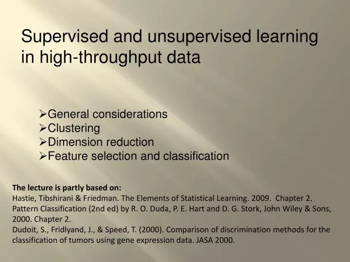
Supervised and u nsupervised learning in high-throughput data

1. Supervised and unsupervised learning in high-throughput data • General considerations • Clustering • Dimension reduction • Feature selection and classification The lecture is partly based on: Hastie, Tibshirani & Friedman. The Elements of Statistical Learning. 2009. Chapter 2. Pattern Classification (2nd ed) by R. O. Duda, P. E. Hart and D. G. Stork, John Wiley & Sons, 2000. Chapter 2. Dudoit, S., Fridlyand, J., & Speed, T. (2000). Comparison of discrimination methods for the classification of tumors using gene expression data. JASA 2000.

2. General considerations This is the common structure of microarray gene expression data from a simple cross-sectional case-control design. Data from other high-throughput technology are often similar.

3. General considerations Supervised learning In supervised learning, the problem is well-defined: Given a set of observations {xi, yi}, estimate the density Pr(Y|X) Usually the goal is to find the location parameter that minimize the expected error at each x: Objective criteria exists to measure the success of a supervised learning mechanism: Error rate from testing (or cross-validation) data Disease classification, predict survival, predict cost … …

4. General considerations Unsupervised learning There is no output variable, all we observe is a set {xi}. The goal is to infer Pr(X) and/or some of its properties. When the dimension is low, nonparametric density estimation is possible; When the dimension is high, may need to find simple properties without density estimation, or apply strong assumptions to estimate the density. There is no objective criteria to evaluate the outcome; Heuristic arguments are used to motivate the methods; Reasonable explanation of the outcome is expected from the subjective field of study. Find co-regulated sets, infer hidden regulation signals, infer regulatory networks, …….

5. General considerations Correlation structure There is always correlations between features (genes, proteins, metabolites …) in biological data. This is caused by the intrinsic biological interactions and regulations. The problem is: We don’t know what the correlation structure is (in some cases we have some idea, e.g. DNA) (2) We cannot reliably estimate it because the dimension is too high and there is not enough data

6. General considerations Curse of Dimensionality Bellman R.E., 1961. In p-dimensions, to get a hypercube with volume r, the edge length needed is r1/p. In 10 dimensions, to capture 1% of the data to get a local average, we need 63% of the range of each input variable.

7. General considerations Curse of Dimensionality In other words, To get a “dense” sample, if we need N=100 samples in 1 dimension, then we need N=10010 samples in 10 dimensions. In high-dimension, the data is always sparse and do not support density estimation. More data points are closer to the boundary, rather than to any other data point  prediction is much harder near the edge of the training sample.

8. General considerations Curse of Dimensionality Just a reminder, the expected prediction error contains variance and bias components. Under model: Y=f(X)+ε

9. General considerations Curse of Dimensionality We have talked about the curse of dimensionality in the sense of density estimation. In a classification problem, we do not necessarily need density estimation. Generative model --- care about class density function. Discriminative model --- care about boundary. Example: Classifying belt fish and carp. Looking at the length/width ratio is enough. Why should we care other variables such as shape of fins, or number of teeth?

10. General considerations N<<p problem We talk about “curse of dimensionality” when N is not >>>p. In bioinformatics, usually N<100, and p>1000. How to deal with this N<<p issue? Dramatically reduce p before model-building. Filter genes based on: variation, normal/disease test statistic, projection…… Use methods that are resistant to large numbers of nuisance variables: Support vector machines, random forests, boosting …… Borrow other information: functional annotation, meta-analysis ……

11. The simplest workflow in biomarker study Obtain high-throughput data Unsupervised learning (dimension reduction/clustering) to show that sample from different treatment are indeed separated, and identify any interesting pattern. Feature selection based on testing – find features that are differentially expressed between treatment. FDR is used here. Experimental validation of the selected features, using more reliable biological techniques. (e.g. real-time PCR is used to validate microarray expression data.) Classification model building. From an independent group of samples, measure the feature levels using reliable technique. Find the sensitivity/specificity of the model using the independent data.

12. Clustering Finding features/samples that are similar. Can tolerate n<p. Irrelevant features contribute random noise that shouldn’t change strong clusters. Some false clusters may be due to noise. But their size should be limited.

13. Clustering Hierarchical clustering Start: every data point being one cluster; Joint nearest clusters at each step.

14. Clustering Hierarchical clustering

15. Clustering Hierarchical clustering Average linkage on microarray data. Row: genes Column: samples

16. Clustering Hierarchical clustering Figure 14.12: Dendrogram from agglomerative hierarchical clustering with average linkage to the human tumor microarray data.

17. Clustering K-means Assign cluster membership Find cluster mean Assign cluster membership based on distance to the means N Convergence? Y Report clusters

18. Clustering K-means How to decide the number of clusters? If there are truly k* groups, for k<k*, some groups are merged, and within-cluster dissimilarity should be big; it should drop substantially when increasing k; when k>k*, some true groups are partitioned. Increasing k should not bring much improvement on within-cluster dissimilarity. Figure 14.8: Total within cluster sum of squares for K-means clustering applied to the human tumor microarray data.

19. PCA PCA sequentially seeks the subspace that explain the most variation in the data. From the covariance matrix: Find the eigen values & vectors: By solving the characteristic equation: Figure 14.20: The first linear principal component of a set of data. The line minimizes the total squared distance from each point to its orthogonal projection onto the line.

20. PCA Figure 14.21: The best rank-two linear approximation to the half-sphere data. The right panel shows the projected points with coordinates given by U2D2, the first two principal components of the data.

21. Classification Fisher Linear Discriminant Analysis Find the lower-dimension space where the classes are most separated.

22. Between class distance Within-class scatter Classification • In the projection, two goals are to be fulfilled: • Maximize between-class distance • Minimize within-class scatter • Maximize this function with all non-zero vectors w

23. Classification Fisher Linear Discriminant Analysis In the two-class case, we are projecting to a line to find the best separation: Maximization yields: mean1 mean2 Decision boundry: Decision boundry

24. Classification Maximum Likelihood discriminant rules Assuming the forms of the class conditional densities are Known. If The rule is Same covariance matrix: Diagonal cov matrix Same diagonal cov matrix across classes

25. Classification Tree An example classification tree.

26. Classification Classification Trees Every split (mostly binary)should increase node purity. Drop of impurity as a criteria for variable selection at each split. Tree should not be overly complex. May prune tree.

27. Classification Tree Choice or features.

28. Classification Random forests Grow an ensemble of classification trees, each based on a bootstrap sample from the original training data. In each tree, the splitter at each node is determined partially at random. Prediction is made by taking the votes from the ensemble of trees. The random forest is a strong classifier; it can help estimate the importance of variables; it helps detect variable interactions.

29. Random Forest

30. Classification Boosting Sequentially apply a weak classification algorithm to reweighted data. The final strong classifier is made from a weighted voting from the weak classifiers.

31. Boosting “A Tutorial on Boosting”,Yoav Freund and Rob Schapire

32. Boosting “A Tutorial on Boosting”,Yoav Freund and Rob Schapire

33. Boosting “A Tutorial on Boosting”,Yoav Freund and Rob Schapire

34. Boosting “A Tutorial on Boosting”,Yoav Freund and Rob Schapire

35. Boosting

36. Classification Support Vector Machine Acknowledge two classes may be inseparable using linear boundary. Maximize C, Allow Slack Variables

37. Classification Support Vector Machine In computing SVM, its solution is special that it only involves the inner product of the input features, and hence for transformed features. Thus the transform need not be explicitly specified. Only the kernel function is needed:

38. SVM Polynomial kernel: http://research.microsoft.com/~cburges/papers/svmtutorial.pdf

39. Classification Support Vector Machine Some commonly used kernels: