Chapter 5 Recurrent Networks and Temporal Feedforward Networks

1. Chapter 5Recurrent Networks and Temporal Feedforward Networks 國立雲林科技大學 資訊工程研究所 張傳育(Chuan-Yu Chang ) 博士 Office: ES 709 TEL: 05-5342601 ext. 4337 E-mail: chuanyu@yuntech.edu.tw

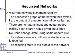
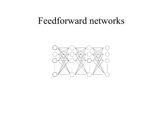
2. Overview of Recurrent Neural Networks • A network that has closed loops in its topological structure is considered a recurrent network. • Feedforward networks: • Implemented fixed-weighted mapping from input space to output space. • The state of any neuron is solely determined by the input to the unit and not the initial and past states of the neuron. • Recurrent neural networks • Recurrent neural networks utilize feedback to allow initial and past state involvement along with serial processing. • Fault-tolerant • These networks can be fully connected. • The connection weights in a recurrent neural network can be symmetric or asymmetric. • In symmetric case, (wij=wji) the network always converges to stable point. However, these networks cannot accommodate temporal sequences of pattern. • In the asymmetric case, (wij≠wji) the dynamics of the network can exhibit limit cycles and chaos, and with the proper selection of weights, temporal spatial patterns can be generated and stored in the network.

3. Hopfield Associative Memory • Hopfield(1988) • The physical systems consisting of a large number of simple neurons can exhibit collective emergent properties. • A collective property of a system cannot emerge from a single neuron, but it can emerge from local neuron interactions in the system. • Produce a content-addressable memory that can correctly yield an entire memory from partial information.

4. Hopfield Associative Memory (cont.) • The standard discrete-times Hopfield neural network • A kind of recurrent network • Can be viewed as a nonlinear associative memory, or content-addressable memory. • To perform a dynamic mapping function. • Intended to perform the function of data storage and retrieval. • The network stores the information in a dynamically stable environment. • A stored pattern in memory is to be retrieved in response to an input pattern that is a noisy version (incomplete) of the stored pattern.

5. Hopfield Associative Memory (cont.) • Content-addressable memory (CAM) • Attractor is a state that the system will evolve toward in time, starting from a set of initial conditions. (basin of attraction) • If an attractor is a unique point in the state space, it is called a fixed point. • A prototype state Fh is represented by a fixed point sh of the dynamic system. • Thus, Fh is mapped onto the stable points sh of the network.

6. Hopfield Associative Memory (cont.)

7. Hopfield Associative Memory (cont.) Activation function: symmetric hard-limiter Output can only be +1 or -1 The output of a neuron is not fed back to itself. Therefore, Wij=0 fori=j.

8. Hopfield Associative Memory (cont.) • The output of the linear combiner is written aswhere is the state of the network • The state of each neuron is given byif vi=0, the value of xj will be defined as its previous state. • The vector-matrix form of (5.1) is given by (5.1) External threshold (5.2) (5.3)

9. Hopfield Associative Memory (cont.) • The network weight matrix W is written asEach row in (5.4) is the associated weight vector for each neuron. • The output of the network can be written asvector-matrix formScalar form (5.4) (5.5) (5.6)

10. Hopfield Associative Memory (cont.) • There are two basic operational phases associated with the Hopfield network: the storage phase and the recall phase. • During the storage phase, the associative memory is build according to the outer-product rule for correlation matrix memories. • Given the set of r prototype memories, the network weight matrix is computed as • Recall phase • A test input vector x’ • The state of network x(k) is initialized with the values of the unknown input, ie., x(0)=x’. • Using the Eq.(5.6), the elements of the state vector x(k) are updated one at a time until there is no significant change in the elements of the vector. When this condition is reached, the stable state xe is the network output. 為了滿足wij=0 fori=j (5.7)

11. Hopfield Associative Memory (cont.) • Discrete-time Hopfield network training algorithm • Step 1: (storage phase) Given a set of prototype memories, using (5.7), the synaptic weights of the network are calculated according to • Step 2: (Recall Phase) Given an unknown input vector x’, the Hopfield network is initialized by setting the state of the network x(k) at time k=0 to x’ • Step 3: The element of the state of the network x(k) are update asynchronously according to (5.6) • This iterative process is continued until it can be shown that the element of the state vector do not change. When this condition is met, the network outputs the equilibrium state (5.8) (5.9) (5.10) (5.11)

12. Hopfield Associative Memory (cont.) • The major problem associated with the Hopfield network is spurious equilibrium state. • These are stable equilibrium states that are not part of the design set of prototype memories. • 造成的spurious equilibrium state原因 • They can result from linear combinations of an odd number of patterns. • For a large number of prototype memories to be stored, there can exist local minima in the energy landscape. • Spurious attractors can result from the symmetric energy function. • Li et al., proposed a design approach, which is based on a system of first-order linear ordinary differential equation. • The number of spurious attractors is minimized.

13. Hopfield Associative Memory (cont.) • Because the Hopfield network has symmetric weights and no neuron self-loop, an energy function (Lyapunov function) can be defined. • An energy function for the discrete-time Hopfield neural network can be written as • The change in energy function is given by x is the state of the network, x’ is an externally applied input presented to the network q is the threshold vector. (5.12) The operation of Hopfield network leads to a monotonically decreasing energy function, and changes in the state of the network will continue until a local minimum of the energy landscape is reached/ (5.13)

14. Hopfield Associative Memory (cont.) (5.14) • For no externally applied inputs, the energy function is given by • The energy change is • The storage capacity (bipolar patterns) of the Hopfield network is approximately by • If most of the prototype memories be recalled perfectly, the maximum storage capacity of the network given by • If it is required that 99% of the prototype memories are to be recalled perfectly n is the number of neurons in the network (5.15) (5.16) (5.17) (5.18)

15. Hopfield Associative Memory (cont.) • Example 5.1 • 有一個具有三個神經元，且權重值為固定，threshold為0的網路架構，因此可有八種可能的輸入(均為bipolar vector) • 網路的權重是由兩個穩定向量(prototype memory) [-1, 1, -1]及[1, -1, 1]根據(5.7)所組成 • 其他的狀態會轉移到此兩個穩定狀態。

16. Hopfield Associative Memory (cont.) • 向量 [-1, -1, 1], [1, -1, -1] 和[1, 1, 1]均會收斂到[ 1, -1, 1] • 利用(5.14)計算能量函數由表5.1可知,在八個可能的輸入中，此兩個穩定的輸入所得到的energy最小。

17. Hopfield Associative Memory (cont.) • Example 5.2 • 每個字母由12*12雙極性值陣列所組成。(+1為黑，-1為白) • 需要12*12=144個神經元，144*144=20736條神經鍵。 • Threshold q=0。 • 每個字母均以向量來表示(-1表黑色、+1表白色)

18. Hopfield Associative Memory (cont.) • 神經鍵的權重值是由5個prototype vector根據(5.7)式所計算求得。如圖5.7所示。 對角線為0 具有30% bit error rate

19. The Traveling-Salesperson Problem • Optimization problems • Finding the best way to do something subject to certain constraints. • The best solution is defined by a specific criterion. • In many cases optimization problems are described in terms of a cost function. • The Traveling-Salesperson Problem, TSP • A salesperson must make a circuit through a certain number of cities. • Visiting each city only once. • The salesperson returns to the starting point at the end of the trip. • Minimizing the total distance traveled.

20. The Traveling-Salesperson Problem (cont.) • Constraint • Weak constraint • Eg. Minimum distance • Strong constraint • Constraints that must be satisfied. • The Hopfield network is guaranteed to converge to a local minimum of the energy function. • To use the Hopfield memory for optimization problems, we must find a way to map the problem onto the network architecture. • The first step is to develop a representation of the problems solutions that fit an architecture having a single array of PEs.

21. The Traveling-Salesperson Problem (cont.) • 以Hopfield解最佳化問題的步驟 • 決定問題設計變數 • 決定問題設計限制及設計目標 • 選擇神經元的狀態表現變數 • 定義能量函數(Lyapunov energy function) ，其最低值，對應網路的最佳解。 • 由能量函數推導出網路的連結權重W，和門限值q • 經由網路的疊代過程，以求得解答。

22. 1 2 3 4 5 A B C D E The Traveling-Salesperson Problem (cont.) • An energy function must satisfies the following criteria. • Visit each city only once on the tour • Visit each position on the tour in a time • Include all n cities. • The shortest total distances.

23. The Traveling-Salesperson Problem (cont.) 每一次只去一個城市 • The energy equation is 每一城市只去一次 從某城市出發，最後回到原出發城市的路徑總浬程最短 所有的N個城市都要去

24. The Traveling-Salesperson Problem (cont.) • Comparing the cost function and the Lyapunov function of the Hopfield networks, the synaptic interconnection strengths and the bias input of the network are obtained as where the Kronecker delta function defined as .

25. The Traveling-Salesperson Problem (cont.) • The total input to neuron (x,i) is

26. A Contextual Hopfield Neural Networks for Medical Image Edge Detection 張傳育(Chuan-Yu Chang) Optical Engineering, vol. 45, No. 3, pp. 037006-1~037006-9,2006. (EI、SCI)

27. Introduction • Edge detection from medical images(such as CT and MRI) is an important steps in the medical image understanding system.

28. Introduction Chang’s[2000]- CHEFNN • The Proposed CHNN • The input of CHNN is the original two-dimensional image and the output is an edge-based feature map. • Taking each pixel’s contextual information. • Experimental results are more perceptual than the CHEFNN. • The execution time is fast than the CHEFNN • The CHEFNN • Advantage: • --Taking each pixel’s contextual information. • --Adoption of the competitive learning rule. • Disadvantage: • -- predetermined parameters A and B, obtain by trial and errors • -- Execution time is long, 26 second above.

29. The Contextual Hopfield Neural Network, CHNN The architecture of CHNN

30. The CHNN • The total input to neuron (x,i) is computed as • The activation function in the network is defined as (1) (2)

31. The CHNN • Base on the update equation, the Lyapunov energy function of the two dimensional Hopfield neural network as (3)

32. The CHNN • The energy function of CHNN must satisfy the following conditions: • The gray levels within an area belonging to the non-edge points have the minima Euclidean distance measure. (4) where (5)

33. The CHNN • The neighborhood function (6) (7)

34. The CHNN • The objective function for CHNN (8)

35. The CHNN • Comparing the objection function of the CHNN in Eq.(8) and the Lyapunov function Eq.(3) of the CHNN (9) (10) (11)

36. The CHNN Algorithm • Input: The original image X, the neighborhood parameters p and q. • Output: The stabilized neuron representing the classified edge feature map of the original image.

37. The CHNN Algorithm • Algorithm: • Step 1) Assigning the initial neuron states as 1. • Step 2) Use Eq.(11) to calculate the total input of each neuron . • Step 3) Apply the activation rule given in Eq.(2) to obtain the new output states for each neuron. • Step 4) Repeat Step 2 and Step 3 for all neurons and count the number of neurons whose state is changed during the updating. If there is a change, then go to Step 2. Otherwise, go to Step 5. • Step 5) Output the final states of neurons that indicate the edge detection results.

38. Experimental Results Phantom images (a) Original phantom image (b) added noise (K=18), (c) added noise (K=20), (d) added noise (K=23), (e) added noise (K=25), (f) noise (K=30)

39. Experimental Results • Noiseless phantom image. • Laplacian-based, • (b) the Marr-Hildreth’s, • (c) the wavelet-based, • (d) the Canny’s, • (e) the CHEFNN, • (f) the proposed CHNN.

40. Experimental Results • Noise phantom image(K=18). • Laplacian-based, • (b) the Marr-Hildreth’s, • (c) the wavelet-based, • (d) the Canny’s, • (e) the CHEFNN, • (f) the proposed CHNN.

41. Experimental Results • Noise phantom image(K=20). • Laplacian-based, • (b) the Marr-Hildreth’s, • (c) the wavelet-based, • (d) the Canny’s, • (e) the CHEFNN, • (f) the proposed CHNN.

42. Experimental Results • Noise phantom image(K=23). • Laplacian-based, • (b) the Marr-Hildreth’s, • (c) the wavelet-based, • (d) the Canny’s, • (e) the CHEFNN, • (f) the proposed CHNN.

43. Experimental Results • Noise phantom image(K=25). • Laplacian-based, • (b) the Marr-Hildreth’s, • (c) the wavelet-based, • (d) the Canny’s, • (e) the CHEFNN, • (f) the proposed CHNN.

44. Experimental Results • Noise phantom image(K=30). • Laplacian-based, • (b) the Marr-Hildreth’s, • (c) the wavelet-based, • (d) the Canny’s, • (e) the CHEFNN, • (f) the proposed CHNN.

45. Experimental Results

46. Experimental Results Knee joint based MR image

47. Experimental Results Skull-based CT image

48. Conclusion • Proposed a new contextual Hopfield neural networks called Contextual Hopfield Neural Network (CHNN) for edge detection. • CHNN considers the contextual information of pixels. • The results of our experiments indicate that CHNN can be applied to various kinds of medical image segmentation including CT and MRI.

49. Recommended Reading • Chuan-Yu Chang and Pau-Choo Chung, “Two-layer competitive based Hopfield neural network for medical image edge detection,” Optical Engineering, Vol. 39, No. 3, pp.695-703, March. 2000. (SCI) • Chuan-Yu Chang, and Pau-Choo Chung, “Medical Image Segmentation Using a Contextual-Constraint Based Hopfield Neural Cube,” Image and Vision Computing, Vol 19, pp. 669-678, 2001. (SCI) • Chuan-Yu Chang, "Spatiotemporal-Hopfield Neural Cube for Diagnosing Recurrent Nasal Papilloma," Medical & Biological Engineering & Computing, Vol. 43. pp. 16-22, 2005(EI、SCI). • Chuan-Yu Chang, “A Contextual-based Hopfield Neural Network for Medical Image Edge Detection,” Optical Engineering, vol. 45, No. 3, pp. 037006-1~037006-9,2006. (EI、SCI) • Chuan-Yu Chang, Hung-Jen Wang and Si-Yan Lin, “Simulation Studies of Two-layer Hopfield Neural Networks for Automatic Wafer Defect Inspection,” Lecture Notes in Computer Science 4031, pp. 1119 – 1126, 2006.(SCI)

50. Simulated Annealing • 由於Hopfield neural network在回想的過程(recalling stored pattern)可能會落入所謂的local minima。但是，在optimization problem上我們希望能夠得到global minimum。 • 因為Hopfield neural network是採用gradient descent法，因此在網路收斂的過程會卡在一個local minimum。 • 所以我們必須在網路的收斂過程中適當的加入一些擾亂，來增加其收斂到global minimum的機率。 • SA可用來解決像是組合最佳化、NP-complete的問題。 • SA與傳統的最陡坡降法不同，因為其在收斂的過程加入了一個擾動量，允許系統跳離local minimum，並持續尋找最佳解 (global minimum) 。 • SA過程包含兩個階段： • Melting the system to be optimized at an effectively high temperature. • Lowering the temperature in slow stages until the system freezes.