Download
1 / 46
460 likes | 593 Views
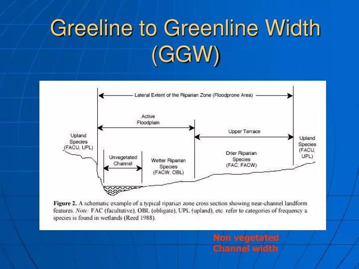
Greeline to Greenline Width (GGW). Non vegetated Channel width. GGW. The non-vegetated distance between the greenlines on each side of the stream. Using “Greenline rules” adds precision to the measurement Consistent GGW measurements between observers validates the greenline rules.

E N D
Greeline to Greenline Width (GGW) Non vegetated Channel width
GGW • The non-vegetated distance between the greenlines on each side of the stream. • Using “Greenline rules” adds precision to the measurement • Consistent GGW measurements between observers validates the greenline rules
Why take out the Vegetated Islands? GGW approximates the scoured, or non-vegetated width of the channel. Including islands adds width bias to the estimate. Typically, we are estimating the width of the “active” channel which normally excludes vegetated bars and islands.
A C B Excludes veg B A Includes bar
B Exclude Vegetation
Using a Laser Range Finder Measures Horizontal Distance (Accuracy - .01 meter) D Ө GGW = cos D Ө x
Long Tom CreekGGW Upstream – light impacts- 4m wide Downstream – heavy impacts – 8 m wide 2007
Long Tom - Spatial Variability Channelshape N = 125 each side alpha = .05
Conclusions - GGW • Reasonably unbiased: measured data • Repeatable: Precision +- 5% • Accurate: Alpha = .05 with sample sizes of from 50 to 100 • Fast: <1 hour with laser range finder, 1.5 hours with rod
Streambank Uncovered/ Unstable (UU) Scour Line Streambank Stability Frame On Greenline
What are streambanks? Streambanks That portion of the channel cross section: - above the scour line, and - below the lip of the first bench.
Scour Line: The lower elevational limit of a streambank. On erosionsal banks, the scour line is the elevation of seasonal scour – often marked by undercut sod.
Bank Scour line Scour line: On depositional banks, the scour line is the lower limit of sod-forming or perennial vegetation – or the potential lower limit of sod-forming vegetation
Top of Bank – lip of first bench Bank Bank Scour line What is the streambank evaluated? Above the Scour Line and at the steepest angle to the water surface. On erosional banks the measurement extends up to the bench or top of cutbank. On bars, it extends up to the top of the depositional feature: approximately bankfull level
First Bench Scour Line The first bench is the first relatively flat area above the scour line or edge of the water
Step 1 Depositional or Erosional? • Depositional: deposited bars – Point bars, lateral bars • Erosional: all other banks
Step 2 Covered or Uncovered • Covered: at least 50% foliar cover of perennial vegetation (including roots); at least 50% cover of cobbles six inches or larger; at least 50% cover of anchored large woody debris (LWD) with a diameter of four inches or greater; • Uncovered: applies to all banks that are not “Covered” as defined above.
Erosional (E) Uncovered (U) Depositional (D) Covered (C)
Step 3 IF “Erosional”, are any of the following present…. Fracture: a visiblecrack is observed. The fracture has not separated into two separate components or blocks of a bank. Cracks indicate a high risk of breakdown. The fracture feature must be at least ¼ of a frame length or greater than about 13 cm of bank length. Slump: streambank that has obviously slipped down resulting in a separate block of soil/sod separated from the bank. Slough or “sluff soil material has fallen from and accumulated near the base of the bank. “Slough” typically occurs on banks that are steep and bare. Eroding: applies to banks that are bare and steep (within 10 degrees of vertical), usually located on the outside curves of meander bends in the stream.
Slumps Fracture
Erosional (E) Uncovered (U) Slough (SL) Depositional (D) Covered (C)
Trampling by large herbivores has caused obvious “slumping.” The slump is greater than one-fourth of the plot length and is recorded (S).
There is a hoofprint in the bank, but no slump or slough is associated with the hoofprint; therefore, there is no indicator of instability so covered (C) and absent (A) are recorded.
Top of bank Scour line Where is the top of the bank? Where is the scour line?
What about entrenched channels? The key: whether slough enters the stream Where is the first Bench?
Lisle (1987) suggested a quick method for measuring pool frequency and residual depth: • Measure distance between depth measurements along the thalweg. • At thalweg depth measurements note the habitat (pool or riffle crest) • To compute residual depth subtract depth at riffle crests from maximum pool depth • The pool frequency is the number of pools per distance along the thalweg.
Potential Indicator of fish habitat quality • Pools are vital components of fish habitat in streams, especially for larger fish • Mossop and Bradford (2006) found a positive correlation between mean maximum residual pool depth and the density of Chinook salmon
Influenced by grazing disturbances In a review of the literature, Powell et al. (2000) concluded that channel characteristics, including channel width and depth, as well as bed material were often reported to be affected by livestock grazing in riparian areas.
Testing Repeatability • Conducted 4 tests in 2009 • Little Truckee (9 crews) • SF Beaver (4 crews) • Summit Creek (6 crews) • Smith Creek (3 crews)
Little Truckee River • Pool structure – Complex • RESIDUAL DEPTH • Average Difference between observers = .01 meter • Maximum Difference = .13 meters • Coefficient of variation (SD/Mean) = 24% • POOLS PER MILE • Average Difference between observers = 12 per mile • Maximum Difference = 21 per mile • CV = 16%
Smith Creek • POOL STRUCTURE - simple • RESIDUAL DEPTH • Average Difference between observers = .01 meter • Maximum Difference = .1 meters • Coefficient of variation (SD/Mean) = 11% • POOLS PER MILE • Average Difference between observers = 7 per mile • Maximum Difference = 10 per mile • CV = 16%
Substrate Size distribution and Percent Fines
Substrate • Channel instability often leads to channel widening, where the energy balance between erosion and deposition shifts toward deposition and therefore fining of the substrate (Powell et al. 2000). • Such increases in fines may degrade aquatic habitat by restricting the living spaces of substrate-dwelling organisms and by limiting the oxygen transfer to incubating eggs (Powell et al. 2000)
Substrate • Pebble counting is a relatively efficient way to measure substrate size distributions and percent fines • Site variability can be problematic. Pebble counts normally detect change when relatively high magnitude impacts are evaluated. The confidence interval is 11% using 200 particles minimum per site. The confidence interval narrows with more particles.
Tendancy to underestimate percent fines • As noted by Bunte and Abt (2001), using different methods to sample substrate at the same location may yield different results. Thus trend over time should be based upon the same technique applied to each sampling event.
Spatial variability • Sampling the entire length of the DMA (20 channel widths) is recommended to ensure spatial variability is accounted for in the sample scheme. If not, variability through time may reflect spatial heterogeneity more than actual adjustments in substrate size distributions.
Substrate Size Distribution At 20 plot locations (200 samples) Sampled between the greenlines 10 particles per plot (cross section) selected at heel and toe across the channel from greenline to greenline – total 200 particles Can lay measuring rod across small streams to obtain sampling intervals
Source • The guidelines on bed material sampling provided by Bunte and Abt (2001) include an excellent summary of the literature and the principal base reference for this protocol.
Why the Substrate Template? “Operator training is extremely important. When selecting particles from a predefined streambed location, or even when measuring particle sizes in a preselected sample of rocks, there is less variability between the results of experienced operators than between those obtained by novices. Field personnel need to be trained to perform procedures accurately, to avoid bias, and to use equipment that reduces operator induced error.” (Bunte and Abt (2001)