Download

1 / 45
460 likes | 641 Views
Marian Scott TIES course January 2012. Introduction to spatial modelling. Outline. Geostatistics Areal unit data Spatial point processes. 1. Geostatistical data. Consider a variable of interest that you wish to measure.

E N D
Marian Scott TIES course January 2012 Introduction to spatial modelling
Outline • Geostatistics • Areal unit data • Spatial point processes
1. Geostatistical data • Consider a variable of interest that you wish to measure. • This variable can be measured at any location within a fixed geographical region A. • However, due to time/cost constraints measurements are only made at n locations u1,…, un. • The measurements (or data) at all n locations are denoted by • Z(u1),…, Z(un) . • Examples of such data include air pollution, temperature, and water quality.
Example – Air pollution Location of the pollution monitors in Greater London.
Goals of geostatistics • Given observations Z(u1),…, Z(un), there are two stages in a general geostatistical analysis. • How do I produce a statistical model for the data? • How do I use my model to estimate quantities of interest such as: • a prediction of Z(u0), where u0 is a location at which Z has not been measured. • a map of Z for the entire region A. • the average value of Z over the region A.
Modelling geostatistical data • When modelling geostatistical data consider the following: • Are the observations Z(u1),….Z(un) Gaussian or do we need to transform them? • Is there a pronounced spatial trend that needs to be modelled – e.g. regression variables or other trends. • Are the responses spatially dependent, i.e. are observations close in space • Similar. • Different. • unrelated.
A general model for the data vector Z=(Z(u1),…, Z(un)), is to represent it as the sum of two components Z = µ + S Where µ is the mean function that models any spatial trend. S is a stochastic process that models spatial dependence. General geostatistical model
Modelling the spatial trend µ • A spatial trend is a smooth change in the average level of the variable Z over the region A. Spatial trends are typically modelled by • Regression variables such as geology or altitude. • Polynomials in the co-ordinates u1…un. • In both cases the mean function can be written as • with known covariates x and unknown parameters β.
Types of spatial dependence • Spatial dependence quantifies how the values of Z(u1),…, Z(un) are related to each other. Three types of spatial dependence are possible. • Independence - the values of Z(u1),…, Z(un) are not related. • Negative dependence – if locations u1 and u2 are close together then Z(u1) and Z(U2) are likely to have different values. • Positive dependence – if locations u1 and u2 are close together then Z(u1) and Z(U2) are likely to have similar values. • The last of these is the most common.
Two common simplifying assumptions are made when modelling positive spatial dependence in geostatistical data. • Stationarity –The spatial dependence between [Z(u0),Z(U1)] is the same as the dependence between [Z(u0+m), Z(U1+m)] for any vector m, i.e. location does not matter. • Isotropy –The dependence between observations at two locations a distance t apart is the same no matter what direction you have to travel to get from the first to the second location, i.e. direction does not matter. • Only the distance between the two points matters
For the remainder of this course we assume: • positive spatial dependence. • any spatial trend has been removed by the mean function µ. • the spatial dependence is stationary and isotropic.
Modelling spatial dependence • A common model for spatial dependence is given by • S ~ N(0 , σ2C) • which implies • the data are normally distributed. • each observation has the same variance, which is equal to σ2 . • the spatial dependence is determined by the correlation matrix C, whose ijth element tells us how similar Z(ui) and Z(uj) are.
Structure of the correlation matrix • The correlation matrix C typically has the following characteristics. • The diagonal elements equal 1, as they represent the correlation of an observation with itself. • The ijth element of C is close to one if locations ui and uj are close together (positive dependence). • As locations ui and uj get further apart, the ijth element gets closer to zero. • Negative dependence (i.e. negative values in C) is rarely seen in geostatistical data.
As we focus on stationary and isotropic spatial dependence, the correlation between 2 measurements Z(u) and Z(u + m) simplifies to • where the points u and u+m are a distance t apart. Therefore, the correlation between 2 points is a function of the scalar distance t between them. The original locations of the points and the direction between them does not matter. • Therefore modelling spatial dependence requires us to specify a function c(t), which tells us how correlation changes with distance.
Semi-variogram modelling • In classical geostatistics spatial dependence was traditionally modelled in terms of a transformation of the correlation function known as the semi-variogram. This function is given by • There are two methods of estimating the semi-variogram.
Semi-variogram cloud Calculate and plot the semi-variogram cloud, which for all pairs of locations is a plot of against This form gives more than one value γ(t) for each value t, and so gives a scatterplot.
Semi-variogram estimator Instead, the semi-variogram cloud values can be combined for pairs of locations that are similar distances apart. This gives the empirical semi-variogram for any value of t. Here N(t) is the set of points (ui, uj) that are distance t apart. This function is then plotted against t.
The nugget is the limiting value of the semi-variogram as the distance t approaches zero. It quantifies either the amount of instrument measurement error in the data or the amount of variation at smaller spatial scales than the closest two measurements. • The sill is the horizontal asymptote of the variogram if it exists, and represents the overall variance of the observations, σ2. • The range is the distance t* at which the semi-variogram reaches the sill. Pairs of points that are further apart than the sill are uncorrelated.
Semi-variogram models A number of semi-variogram models exist that can be used. Nugget - random data Spherical Exponential Although these models may not fit the data particularly well.
Examples in R • To see how the shape of the semi-variogram corresponds to the smoothness and variation in a spatial surface, we use the R package rpanel for illustration.
Modelling spatial data • This gives us a three stage process by which to model spatial data. • Determine the form of the mean function and subtract it from the observed data to form residuals. • Plot the empirical semi-variogram of the residuals and determine which family of semi-variogram models it resembles. • Estimate the parameters of the mean function and the chosen semi-variogram model (sill, nugget, range) by least squares, maximum likelihood or Bayesian methods.
Modelling in practice • For most real data that you wish to model the empirical semi-variogram will not have the nice shapes seen in the examples, and will not look anything like any of the theoretical semi-variogram models. This will make 2 above difficult (impossible). • A pragmatic strategy is to fit a number of different spatial correlation models and see how the different choices affect your results.
Spatial prediction • Once you have produced a statistical model for the data, prediction of the variable of interest at unmeasured locations u0 is typically of interest. There are many methods for doing this including: • Regression modelling using generalised least squares. • Inverse distance weighted interpolation. • Kriging. • Most of which can be easily implemented in modern statistical packages such as R.
The majority of these approaches predict Z(u0) by a weighted average of the data, i.e. • The main difference between the methods is how the weights are estimated. • A map can be produced by predicting the surface at a regular grid of points across the region A. • The average value across the region A can be estimated by averaging the predictions on this regular grid.
Example - Spatial modelling in R • We now see how to implement these spatial models in R using the package geoR.
2. Areal unit data • Consider a variable that cannot be measured at any location within a geographical region A. • Instead, the variable can be measured as summaries for n non-overlapping sub-regions A1,….,An. • The measurements (data) are denoted by Z1,….Zn. • Examples include • demographic summaries (number of people per county). • aggregated data due to confidentiality (e.g. personal data). • where exact locations are not recorded (e.g. election voting).
Motivating example • The graph shows lip cancer rates for the 56 counties in Scotland. Two possible questions of interest: • Do any environmental variables affect the number of new cases? • Are there areas of Scotland with unusually high levels of lip cancer? • Map taken from a paper by Wakefield from Biostatistics 2007, 158-183.
Modelling areal unit data • When modelling areal unit data Z1,….,Zn from sub-regions A1,…,An you need to consider the following: • Response distribution – is Zi Gaussian, Poisson, binomial, etc. • Mean function – are there any important covariates that can be used in the mean function. For example, sunlight in the lip cancer example. • Spatial dependence – Are the data spatially dependent and if so how should this be modelled?
Modelling spatial dependence • In common with geostatistical data, spatial dependence will typically be positive rather than negative. There are two common methods for modelling this dependence. • Use a geostatistical model as in the previous section, where the locations of Z1,….,Zn are assumed to be the central points of the sub-areas A1,…,An. • Use a model that is based on the notion of a neighbourhood matrix W, that links the n sub-areas.
Neighbourhood matrix W • The “proximity” between each pair of sub-areas Ai,Akcan be summarised by an n by n neighbourhood matrix W, which comprises 1’s and 0’s. • Element Wik is 1 if areas i and k are neighbours and 0 otherwise. • Areas Ai,Ak could be neighbours if • they share a common border. • are less than a distance d apart. • are one of the closest areas in terms of distance. A border specification
Conditional autoregressive models • Using a neighbourhood matrix W, a standard model for areal unit data is called a conditional autoregressive (CAR) model. In its simplest form it is given by specifying the distribution of each Zi, conditional on all the remaining values. • Z-i is the vector including all the elements of Z except the ith. • is the mean of the observations in areas neighbouring area i. • ni is the number of neighbours that area i has.
3. Spatial point processes • Consider a fixed geographical region A. • Spatial point process modelling is used when the set of locations where a particular phenomenon occurs are of interest. • For a given phenomenon the set of locations at which events occur is denoted by u1,…un. So the data here are the locations. • Additional measurements may be made about the phenomenon at each location (marked point process). • Examples include lightning strikes and the locations of trees in a forest.
Question of interest • The key question of interest for spatial point process data is • “Does the observed process have any spatial dependence?” • Three general types of structure are possible. • Complete spatial randomness (CSR) – events occur at random. • Clustered process – events occur close to existing events. • Regular process – events occur away from existing events.
Example 1 The locations of the centres of 42 biological cells observed under an optical microscope.
Example 3 Location of 65 Japanese black pine saplings in a square region of 5.7 metres squared.
How do you tell? • For some of these examples it’s not easy to determine by eye whether they are spatially random, clustered or regular. A more systematic approach for answering this question is to: • Develop a statistical model for complete spatial randomness (CSR), and see if the observations seem likely under that model. • If they are likely then complete spatial randomness can be assumed. • If not then it should be easy to determine whether the point process is clustered or regular.
A model for CSR • Let N(Ak) denote the number of events in a sub-area Ak. • Then CSR asserts that: • (i) For any sub-region Ak, N(Ak)~Poisson(|Ak|). • (ii) For disjoint sub-regions (A1, A2) , N(A1) and N(A2) are independent. • is termed the intensity, and is the expected number of events per unit area. • Therefore |A| is the expected number of events in A. • A process satisfying (i) and (ii) is called a homogeneous Poisson process (with intensity ).
Mean and covariance • For a CSR process on the region A • Mean – The average number of events in a sub-region Ai e.g. E[N(Ai)], does not depend on the location of the sub-region. • Variance – The variance of the number of events in Ai, e.g. Var[N(Ai)], is equal to E[N(Ai)]. • Covariance – The spatial dependence between two observations (u1, u2) is determined by the second order intensity function 2 (u1, u2) . • However the latter is hard to work with.
The K function • Instead of working with the second order intensity function • 2 (u1, u2) to measure spatial dependence, we work with the • K function which is a function of distance t. • K(t) = E{N0(t)} / • = E(number of events within a distance t of U0) / • Here N0(t) is the number of events within a distance t of an existing data point U0. So • for large t, K(t) will be large U0 • for small t, K(t) will be small t
Why is the K function useful? • Recall that • K(t) = E(number of events within a distance t of U0) / • For a CSR process - K(t) = t2 / = t2 - the area of a circle • For a clustered process we would expect more points close together than under CSR, so for small t, K(t) > t2. • For a regular process we would expect less points close together than under CSR, so for small t, K(t) < t2.
Determining whether CSR holds? • Step 1 - estimate the intensity by • hat= N(A)/|A|. • Step 2 - estimate K(t) for a sequence of distances t. • Step 3 – Plot the theoretical function for CSR, K(t) = t2, against t, and add a second line for the estimated K function for the point process. If CSR is reasonable they will be very similar.
Further models for point processes • If CSR does not hold for the data in question there are other models that can be used. For example • Poisson cluster process – Models clusters. • Inhibition process – models regular processes.
Implementing point process models • Point process models (including CRS and others) can be implemented in R using the add on libraries • spatstat • Splancs • For further details see http://lib.stat.cmu.edu/R/CRAN/.