Download
1 / 73
730 likes | 1.03k Views
Chapters 5 and 6: Numerical Integration. Definition of Integral by Upper and Lower Sums. Application to monotone decreasing function. (composite form: equal subintervals). As part of assignment #2 (due 2/4/14), derive the integration

E N D
Definition of Integral by Upper and Lower Sums
Application to monotone decreasing function
As part of assignment #2 (due 2/4/14), derive the integration and error formulas for upper and lower sums applied to a monotone increasing function.
Derivation of trapezoid rule for any f(x) Approach: linear approximation Result obtained using upper and lower sums
Use Taylor formula to derive an expression for the expected error in the trapezoid rule for any function with a continuous second derivative
Single subinterval of size h Fundamental theorem of calculus
n subintervals n+1 points Mean value theorem
Assignment 2, Due 2/4/14 • Use the relationship • Integral = (upper sum + lower sum)/2 • to derive a numerical integration formula for a monotone increasing function. • 2. Use the relationship • Error = (upper sum – lower sum)/2 • to derive an error approximation for the formula derived in (1).
Assignment 2, Due 2/4/14 continued 3. Use the error formulas derived in class for the composite trapezoid rule applied to the integral to obtain 2 estimates of the number of sub-intervals needed to have an error less than 10-4 4. Write a MabLab function for the composite trapezoid rule with function handle and number of subintervals as parameters. Use this code to discover which of the error estimates in (3) is more realistic.
Problems from text on application of error formulas 5.1-6 p188 5.2-2 p 200 5.2-4 p200 5.2-7 p200 5.2-12 p210 6.1-2a p227
Problem 5.1-6 text p 188 If the integral is evaluated by upper and lower sums, estimate the number of points needed for accuracy 0.5x10⁻⁴
Problem 5.2-2 text p 200 Estimate the error if the integral is evaluated by the composite trapezoid rule with 3 points |error| < (b-a)3|f’’(x)|max /12n2 Plot |f’’(x)| to estimate maximum value on [0, 1]
|f’’(x)| X
Problem 5.2-2 text p 200 Estimate the error if the integral is evaluated by the composite trapezoid rule with 3 points |error| < (b-a)3|f’’(x)|max /12n2 = (1)(2)/((12)(9)) = 1/54 Correct answer is 1/24. What is wrong?
For given number of points, accuracy of numerical integration depends on where the integrand is evaluated Accuracy of numerical integration also depends on the variable of integration Consider approximated by the trapezoid rule with (a) equally spaced points in the interval 1<x<5 (b) logarithmically spaced points in the interval 1<x<5 (c) equally spaced points with integration variable y = ln(x) For (b) we need a trap rule that accepts arbitrary spacing
MatLab function: numerical integration with arbitrary spacing
Use the transformation y = ln(x) to change the variable of integration. dy = dx/x x(y)= exp(y) Integrand is a function of y through x(y)
3 trapezoid rule approximations to x(y)= exp(y)
% error Number of points
Assignment 3, Due 2/11/14 On page 242 of text, the value of is given to high precision, which can be taken as the “exact” value. Defined relative error as re = 100|(TR-exact)/exact|, where TR denotes the trapezoid-rule approximation. Write a MATLAB code to compare the relative error with 10 points when the points are chosen in the following ways: 1. Equally space on [1, 3] 2. Log-spaced on [1, 3] 3. Equally space on [0, ln(3)] in the new integration variable y = ln(x).
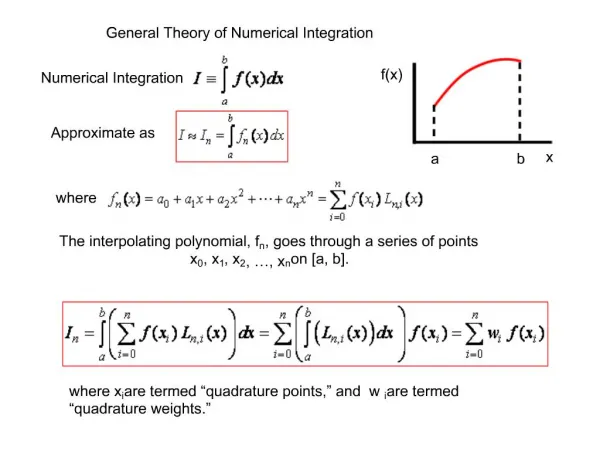
Most numerical integration formulas have the form Example: Trapezoid rule w0 = wn = 1/2n wk = 1/n if 1< k<n-1 n = number of intervals One approach to deriving such formulas: Replace the integrand by the Lagrange interpolation formula
Another example Why is this different from Simpson’s rule?
Which is likely to be more accurate?
Problems from text p240 on deriving integration formulas 6.2-5 6.2-6 6.2-9
Example 6.2-6 text p240 Find A and B by requiring formula to be exact for f(x) = 1 and f(x) = x
Problem 6.1-4 text p228 Evaluated by composite Simpson’s rule with h=0.25 Bound the error |error| = (b-a)h4|f(4)(x)|/180 a <x< b (text p221) h = width subintervals
Let {x0, x1, …, xn} be n+1 points on [a, b] where integrand evaluated. Will be exact for polynomials of degree n Trapezoid rule: (n = 1) exact for a line In general, error proportional to |f’’(z)| Simpson’s rule: (n = 2) exact for a parabola In general, error proportional to |f(4)(z)| How could this happen?
Gauss quadrature extents Simpson’s rule idea to its logical extreme: Give up all freedom about where the integrand will be evaluated to maximize the degree of polynomial for which formula is exact. nodes {x0, x1, …, xn} exist on [a, b] such that is exact for polynomials of degree at most 2n+1 Nodes are zeros of polynomial g(x) of degree n+1 defined by 0 < k < n
Summary of Gauss Quadrature Theorem For any set of n+1 nodes on [a,b], is exact for polynomials up to degree n For the special set of node in Gauss quadrature, the formula is correct of polynomials of degree at most 2n+1 Nodes and weights, Ai, depend on both [a,b] and n Scaling property of integrals lessens the impact of these dependences
Degree of g(x) = number of nodes Number of conditions on g(x) = number of nodes Number of conditions not Sufficient to determine all coefficients Terms with odd powers of x in g(x) do not contribute due to symmetry
Determines ratio of C1 and C3 only. As noted before, number of conditions on g(x) insufficient to determine all 4 coefficients of a cubic
Nodes and weights determined for [-1,1] can be used for [a,b] Given values of y from table, this x(y) determines values on [a,b] where integrand will be evaluated
From text p236 Note: n = number of intervals Example: note symmetry of points and weights
(no anti-derivative) with 2 nodes