1: Basics of optimization-based segmentation - continuous and discrete approaches

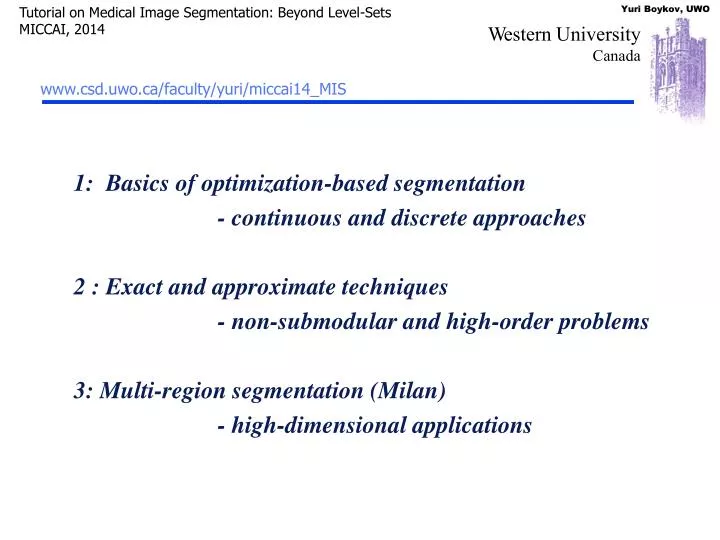
1. Tutorial on Medical Image Segmentation: Beyond Level-Sets MICCAI, 2014 Western University Canada www.csd.uwo.ca/faculty/yuri/miccai14_MIS 1: Basics of optimization-based segmentation - continuous and discrete approaches 2 : Exact and approximate techniques - non-submodular and high-order problems 3: Multi-region segmentation (Milan) - high-dimensional applications

2. Introduction to Image Segmentation • implicit/explicit representation of boundaries • active contours, level-sets, graph cut, etc. • Basic low-order objective functions (energies) • physics, geometry, statistics, information theory • Set functions, submodularity • Exact methods • Approximation methods • Higher-order and non-submodular objectives • Comparison to gradient descent (level-sets) Part 1 Part 2

3. Thresholding T

4. Thresholding T S={ p :Ip < T }

5. Thresholding Background Subtraction ? I= Iobj- Ibkg - = Threshold intensities above T better segmentation?

6. Good segmentation S ? Segmentation becomes an optimization problem: S = arg min E(S) • Objective function must be specified Quality function Cost function Loss function E(S) : 2P  “Energy” Regularization functional

7. Good segmentation S ? • Objective function must be specified Quality function Cost function Loss function E(S) = E1(S)+…+ En(S) “Energy” Regularization functional combining different constraints e.g. on region and boundary Segmentation becomes an optimization problem: S = arg min E(S)

8. Beyond linear combination of terms Not in this tutorial • Ratios are also used • Normalized cuts [Shi, Malik, 2000] • Minimum Ratio cycles [JarminIshkawa, 2001] • Ratio regions [Cox et al, 1996] • Parametric max-flow applications [Kolmogorov et al 2007]

9. Segmentation principles interactive vs. unsupervised • Normalized cuts [Shi Malik] • Mean-shift [Comaniciu] • MDL [Zhu&Yuille] • Entropy of appearance • Add enough constraints: • Saliency • Shape • Known appearance • Texture • Boundary seeds • Livewire (intelligent scissors) • Region seeds • Graph cuts (intelligent paint) • Distance (Voronoi-like cells) • Bounding box • Grabcut [Rother et al] • Center seeds • Star shape [Veksler] • Many other options…

10. 1. We won’t cover everything… 2. We will not emphasize the differences between interactive and unsupervised (too easy to convert one into the other) interactive vs. unsupervised • Normalized cuts [Shi Malik] • Mean-shift [Comaniciu] • MDL [Zhu&Yuille] • Entropy of appearance • Add enough constraints: • Saliency • Shape • Known appearance • Texture • Boundary seeds • Livewire (intelligent scissors) • Region seeds • Graph cuts (intelligent paint) • Distance (Voronoi-like cells) • Bounding box • Grabcut [Rother et al] • Center seeds • Star shape [Veksler] • Many other options…

11. Common segmentation techniques boundary-based region-based both region & boundary • thresholding • geodesic • active contours • (e.g. level-sets) • MRF • (e.g. graph-cuts) • random walker optimization-based region-growing intelligent scissors (live-wire) active contours (snakes) watersheds

12. Common surface representations continuous optimization mixed optimization combinatorial optimization graph labeling point cloud labeling level-sets mesh on complex on grid

13. Active contours (e.g. snakes) • [Kass, Witkin, Terzopoulos 1987] Given: initial contour (model) near desirable object Goal: evolve the contour to fit exact object boundary

14. Tracking via active contours Tracking Heart Ventricles

15. Active contours - snakesParametric Curve Representation (continuous case) A curve can be represented by 2 functions parameter closed curve open curve

16. Snake Energy internal energy encourages smoothness or any particular shape external energy encourages curve onto image structures (e.g. image edges)

17. Active contours - snakes (continuous case) • internal energy (physics of elastic band) • external energy (from image) elasticity / stretching stiffness / bending proximity to image edges

18. Active contours – snakes (discrete case) elastic energy (elasticity) bending energy (stiffness)

19. Basic Elastic Snake continuous case discrete case elastic smoothness term (interior energy) image data term (exterior energy)

20. Snakes - gradient descent C simple elastic snake energy here, energy is a function of 2n variables C update equation for the whole snake

21. Snakes - gradient descent C simple elastic snake energy here, energy is a function of 2n variables C update equation for each node

22. Snakes - gradient descent E(C) energy function E(C) for contours C gradient descent steps local minima for E(C) step size could be tricky second derivative of image intensities

23. Implicit (region-based) surface representation via level-sets (implicit contour representation) [Dervieux, Thomasset, 79, 81] [Osher, Sethian, 89]

24. The scaling by is easily verified in one dimension Implicit (region-based) surface representation via level-sets Normal contour motion can be represented by evolution of level-set function u [Dervieux, Thomasset, 79, 81] [Osher, Sethian, 89] Note 1: - commonly used for gradient descent evolution Note 2: - level sets can not represent tangential motion of contour points ???

25. Tangential vs. normal motion of contour points - normal motion of a contour point visibly changes shape (geometry) - tangential motion generates no “visible” shape change A simple example of tangential motion of contour points (rotation) A simple example of normal motion of contour points (expansion) Comments: - geometric “energy” of a contour measures “visible” shape properties (length, curvature, area, e.t.c.). Thus, gradient descent w.r.t. geometric objective generates only ”visible” (normal) motion. • level sets can represent contour gradient descent evolution • only for geometric “energies” E(C) (s.t. E is collinear with contour normal ) Level sets (implicit contour representation) Geodesic active contours

26. Tangential vs. normal motion of contour points - normal motion of a contour point visibly changes shape (geometry) - tangential motion generates no “visible” shape change Q: in what medical applications tangential motion of segment boundary matters? Comments: - gradient descent for physics-based “energy” of a contour (e.g. elasticity) may produce geometrically “invisible” tangential motion of contour points • physics-based energy of a contour depends on its parameterization, • while geometrically it could be the same contour (compare two shapes above) Parametric contours (explicit contour representation) Physics-based active contours

27. Physics vs. Geometry continuous optimization mesh level-sets • geodesic active contours • implicit or non-parametric representation • geometry-based objectives • gradient descent • can use convex formulations (TV-based) • snakes, balloons, active contours • explicit or parametric contour representation • physics-based objectives (typically) • gradient descent • could use dynamic programming in 2D [Amini, Weymouth, Jain, 1990] [Chan, Esidoglu, Nikolova 2006]

28. Most common geometric functionals for segmentation with level-sets Functional E( C ) or weighted length (boundary alignment to intensity edges) weighted area (region alignment to appearance model) flux (oriented boundary alignment)

29. Most common geometric functionals for segmentation with level-sets Functional E( C ) or weighted length (boundary alignment to intensity edges) weighted area (region alignment to appearance model) flux (oriented boundary alignment)

30. B A Towards discrete geometry:weighted boundary length on a graph [Barrett and Mortensen 1996] “Live wire” or “intelligent scissors” pixels image-based edge weights | I| shortest path algorithm (Dijkstra)

31. Graph Cuts approach Shortest paths approach p Compute the shortest pathp ->p for a point p. shortest path on a 2D graph graph cut Example: find the shortest closed contour in a given domain of a graph Compute the minimum cut that separates red region from blue region Repeat for all points on the gray line. Then choose the optimal contour.

32. B A A Path connects points A Cut separates regions graph cuts vs. shortest paths • On 2D grids graph cuts and shortest paths giveoptimal 1D contours. • Shortest paths still give optimal 1-D contours on N-D grids • Min-cuts give optimal hyper-surfaces on N-D grids

33. a cut hard constraint n-links hard constraint t s Graph cut [Boykov and Jolly 2001] Minimum cost cut can be computed in polynomial time (max-flow/min-cut algorithms)

34. Minimum s-t cuts algorithms • Augmenting paths [Ford & Fulkerson, 1962] • - heuristically tuned to grids [Boykov&Kolmogorov 2003] • Push-relabel[Goldberg-Tarjan, 1986] • - good choice for denser grids, e.g. in 3D • Preflow [Hochbaum, 2003] • - also competitive

35. Optimal boundary in 2D “max-flow = min-cut”

36. Optimal boundary in 3D 3D bone segmentation (real time screen capture, year 2000)

37. (discrete geometry) NOTE: many distance-to-seed methods optimize segmentation boundary only indirectly, they compute some analogue of optimum Voronoi cells [fuzzy connectivity, random walker, geodesic Voronoi cells, etc.] ‘Smoothness’ of segmentation boundary - snakes (physics-based contours) - geodesic contours (geometry) - graph cuts

38. Geodesic contours Discrete vs. continuous boundary cost Graph cuts Both incorporate segmentation boundary smoothness and alignment to image edges C [Caselles, Kimmel, Sapiro, 1997] (level-sets) [Boykov and Jolly 2001] [Chan, Esidoglu, Nikolova, 2006] (convex) [Boykov and Kolmogorov 2003]

39. Graph cuts on a grid and boundary of S • Severed n-links can approximate geometric length of contour C [Boykov&Kolmogorov, ICCV 2003] • This result fundamentally relies on ideas of Integral Geometry(also known asProbabilistic Geometry)originally developed in 1930’s. • e.g.Blaschke, Santalo, Gelfand

40. a subset of lines L intersecting contour C a set of all lines L Euclidean length of C : Cauchy-Crofton formula the number of times line L intersects C Integral geometry approach to length C probability that a “randomly drown” line intersects C

41. C Edges of any regular neighborhood system generate families of lines { , , , } Euclidean length graph cut cost for edge weights: the number of edges of family k intersecting C Graph cuts and integral geometry Graph nodes are imbedded in R2 in a grid-like fashion Length can be estimated without computing any derivatives

42. Metrication errors Euclidean metric “standard” 4-neighborhoods (Manhattan metric) 8-neighborhoods larger-neighborhoods Riemannian metric

43. 4-neighborhood Metrication errors 8-neighborhood

44. Differential vs. integral approach to geometric boundary length Parametric (explicit) contour representation Differential geometry Level-set function representation Integral geometry Cauchy-Crofton formula implicit (region-based) representation of contours

45. Level set function u(p) is normally stored on image pixels • Values of u(p) can be interpreted asdistancesorheights of image pixels -0.8 -0.8 -1.7 0.2 A contour may be approximated from u(x,y) with sub-pixel accuracy -0.5 0.5 -0.6 -0.4 0.7 -0.2 0.3 0.6 Implicit (region-based) surface representation via level-sets C

46. 0 0 0 1 There are many contours satisfying interior/exterior labeling of points 0 1 0 0 Question: Is this a contour to be reconstructed from binary labeling Sp? 1 0 1 1 Implicit (region-based) surface representation via graph-cuts • Graph cuts represent surfaces via binary labeling Spof each graph node • Binary values of Spindicate interioror exterior points (e.g. pixel centers) C Answer: NO

47. Contour/surface representations(summary) Implicit (area-based) Explicit (boundary-based) Snakes (physics-based band model) Level sets (geodesic active contours) Live-wire (shortest paths on graphs) Graph cuts (minimum cost cuts) What else besides boundary length |∂S| ?

48. a cut n-links t-link t t-link assume are known “expected” intensities of object and background s From seeds to more general region constraints [Boykov and Jolly 2001] S segmentation cost of severed t-links cost of severed n-links E(S) = +

49. a cut n-links t-link t t-link could be unknown intensities of object and background s From seeds to more general region constraints [Boykov and Jolly 2001] S re-estimate segmentation cost of severed t-links cost of severed n-links Block-Coord.Descent E(S, Is,It) = + Chan-Vese model

50. Block-coordinate descent for optimal L can be computed using graph cuts fixed for S=const optimal I 1, I 0 can be computed by minimizing squared errors inside object and background segments Minimize over labeling S for fixed I0, I1 Minimize over I0, I1 for fixed labeling S