Mid-course overview (NB: overview a guide but not necessarily everything)

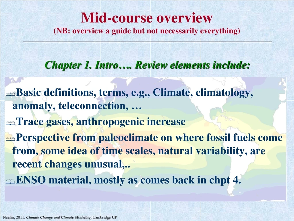
1. Basic definitions, terms, e.g., Climate, climatology, anomaly, teleconnection, … Trace gases, anthropogenic increase Perspective from paleoclimate on where fossil fuels come from, some idea of time scales, natural variability, are recent changes unusual,.. ENSO material, mostly as comes back in chpt 4. Mid-course overview(NB: overview a guide but not necessarily everything) Chapter 1. Intro…. Review elements include: Neelin, 2011. Climate Change and Climate Modeling, Cambridge UP

2. Climate: average condition of the atmosphere, ocean, land surfaces and the ecosystems in them (includes average measures of weather-related variability, e.g. storm frequency) Weather: state of atmosphere and ocean at given moment. Average taken over January of many different years to obtain a climatological value for January, etc. 1.1 Climate dynamics, climate change and climate prediction Neelin, 2011. Climate Change and Climate Modeling, Cambridge UP

3. Climate change: occurring on many time scales, including those that affect human activities. time period used in the average will affect the climate that one defines. e.g., 1950-1970 will differ from the average from 1980-2000. Climate variability: essentially all the variability that is not just weather. e.g., ice ages, warm climate at the time of dinosaurs, drought in African Sahel region, and El Niño. Neelin, 2011. Climate Change and Climate Modeling, Cambridge UP

4. Global warming: predicted warming, & associated changes in the climate system in response to increases in "greenhouse gases" emitted into atmosphere by human activities. Greenhouse gases: e.g., carbon dioxide, methane and chlorofluorocarbons: trace gases that absorb infrared radiation, affect the Earth's energy budget. warming tendency, known as the greenhouse effect Climate prediction endeavor to predict not only human-induced changes but the natural variations. e.g., El Niño Climate models: Mathematical representations of the climate system typically equations for temperature, winds, ocean currents and other climate variables solved numerically on computers. Neelin, 2011. Climate Change and Climate Modeling, Cambridge UP

5. El Niño: largest interannual (year-to-year) climate variation interaction between the tropical Pacific ocean and the atmosphere above it. a prime example of natural climate variability. first phenomenon for which the essential role of dynamical interaction between atmosphere and ocean was demonstrated. Neelin, 2011. Climate Change and Climate Modeling, Cambridge UP

6. Teleconnections: remote effects of El Niño (or other regional climate variations). Anomaly:departure from normal climatological conditions. calculated by difference between value of a variable at a given time, e.g., pressure or temperature for a particular month, and subtracting the climatology of that variable. Climatology includes the normal seasonal cycle. e.g., anomaly of summer rainfall for June, July and August 1997, = average of rainfall over that period minus averages of all June, July and August values over a much longer period, such as 1950-1998. To be precise, the averaging time period for the anomaly and the averaging time period for the climatology should be specified. e.g., monthly averaged SST anomalies relative to 1950-2000 mean. Neelin, 2011. Climate Change and Climate Modeling, Cambridge UP

7. Table 1.1 1.4 Global change in recent history Neelin, 2011. Climate Change and Climate Modeling, Cambridge UP

8. Figure 1.1 Carbon dioxide concentrations since 1958,measured at Mauna Loa, Hawaii. • Annual, interannual variations: • biological impacts on carbon cycle • Trend: due to fossil fuel emissions. Neelin, 2011. Climate Change and Climate Modeling, Cambridge UP

9. Figure 1.2 Concentration of various trace gasesestimated since 1850 • Methane: Cattle, sheep, rice paddies, fossil fuel by-product; wetlands, termites (parts per billion). • Nitrous Oxide: biomass burning, fertilizers? • Chlorofluorocarbons: man-made, zero before 1950 (parts per trillion). Neelin, 2011. Climate Change and Climate Modeling, Cambridge UP

10. Figure 1.3 Global mean surface temperatures estimated since preindustrial times • Anomalies relative to 1961-1990 mean • Annual average values of combined near-surface air temperature over continents and sea surface temperature over ocean. • Curve: smoothing similar to a decadal running average. • From University of East Anglia Climatic Research Unit, Brohan et al. (2006). Neelin, 2011. Climate Change and Climate Modeling, Cambridge UP

11. ENSO: El Niño/Southern Oscillation. [Cont’d in Chpt 4] El Niño is associated with warm phase of a phenomenon that is largely cyclic. La Niña for the cold phase. El Niño arises in tropical Pacific along the equator. Changes in sea surface temperature, ocean subsurface temperatures down to a few hundred meters depth, rainfall, and winds: ocean-atmos. interaction! Variations in the Pacific basin within about 10-15 degrees latitude of the equator are the primary variables. 1.5 El Niño: An example of natural climate variability Neelin, 2011. Climate Change and Climate Modeling, Cambridge UP

12. Figure 1.12 Paleoclimate: A few climate notes with Geological time scale • Very distant past--- Myr=millions of years • Key points: • Climate can vary substantially, on all timescales • Long periods in deep past with warmer climate than present (& higher est. CO2 ) • deposition over 100s of millions of years sequesters carbon dioxide as fossil fuels (oil, coal, natural gas) • return of this CO2 to atmosphere occurring over very short period. Neelin, 2011. Climate Change and Climate Modeling, Cambridge UP

13. Figure 1.13 Antarctic ice core records of CO2, deuterium isotope ratio variations (dD), and Antarctic air temperature inferred from dD Neelin, 2011. Climate Change and Climate Modeling, Cambridge UP

14. Chapter 2 Basics of Global Climate • Review elements include: • Basic concepts and terminology that tend to recur later: • E.g., albedo, moist convection, easterly winds 2.1 Components and phenomena in the climate system • Climate processes • solar radiation tends to get through the atmosphere; ocean heated from above Þ stable to vertical motions. • warm surface layer, colder deep waters • mixing near ocean surface Þupper mixed layer ~ 50 m • mixing carries surface warming down as far as thermocline, layer of rapid transition of temperature to the colder abyssal waters below Neelin, 2011. Climate Change and Climate Modeling, Cambridge UP

15. Figure 2.2 Satellite image based on visible light with 5°x5° grid overlay Courtesy of NASA Neelin, 2011. Climate Change and Climate Modeling, Cambridge UP

16. The parameterization problem • For each grid box in a climate model, only the average across the grid box of wind, temperature, etc. is represented. • The average ofsmaller scale effects has important impacts on large-scale climate. • e.g., clouds primarily occur at small scales, yet the average amount of sunlight reflected by clouds affects the average solar heating of a whole grid box. • Parameterization: representing average effects of scales smaller than the grid scale (e.g., clouds) as a function of the grid scale variables (e.g. temperature and moisture) in a climate model. Neelin, 2011. Climate Change and Climate Modeling, Cambridge UP

17. 2.2 Basics of radiative forcing • Solar radiation input: Infrared radiation (IR) is the only way this heat input can be balanced by heat loss to space • Since IR emissions depend on the Earth's temperature, the planet tends to adjust to a temperature where IR energy loss balances solar input: • Blackbody radiation: approximation for how radiation depends on temperature: • Total energy flux integrated across all wavelengths of light R = sT4 • Full climate models do detailed computation as a function of wavelength, for every level in the atmosphere, … • [& Trace gases absorb IR at wavelengths where O2, N2 ineffective….] Neelin, 2011. Climate Change and Climate Modeling, Cambridge UP

18. 2.3 Globally averaged energy budget Pathways of energy transfer in a global average Figure 2.8 Neelin, 2011. Climate Change and Climate Modeling, Cambridge UP

19. Greenhouse effect: • The upward IR from the surface is mostly trapped in the atmosphere, rather than escaping directly to space, so it tends to heat the atmosphere. • The atmosphere warms to a temperature where it emits sufficient radiation to balance the heat budget, but it emits both upward and downward, so part of the energy is returned back down to the surface where it is absorbed. • This results in additional warming of the surface, compared to a case with no atmospheric absorption of IR. • Atmosphere emits IR downward Þ absorbed at surface. • Both gases and cloudscontribute to absorption of IR and thus to the greenhouse effect. Neelin, 2011. Climate Change and Climate Modeling, Cambridge UP

20. Pathways of energy transfer in a global average (cont.) • At the top of the atmosphere, in the global average and for a steady climate: • IR emitted balances incoming solar. • Global warming involves a slight imbalance: • a change in the greenhouse effectÞ slightly less IR emitted from the top (chap. 6). • small imbalance Þ slow warming. • Three roles for clouds and convection: • heating of the atmosphere (through a deep layer) • reflection of solar radiation (contributing to albedo) • trapping of infrared radiation (contributing to the greenhouse effect) Neelin, 2011. Climate Change and Climate Modeling, Cambridge UP

21. 2.4 Gradients of rad. forcing and energy transport by atm. • Differences in input of solar energy between latitudes Þ temperature gradients. • These gradients would be huge if it were not for heat transport in ocean & atmosphere and heat storage in ocean. Figure 2.9 Neelin, 2011. Climate Change and Climate Modeling, Cambridge UP

22. Latitude structure of the circulation (cont.) • Hadley cell: thermally driven, overturning circulation, rising in the tropics and sinking at slightly higher latitudes (the subtropics). • Explanations of this in chpt. 3 • Relation to observations • rising branch assoc. with convective heating and heavy rainfall; subtropical descent regions, little rain. Neelin, 2011. Climate Change and Climate Modeling, Cambridge UP

23. Figure 2.13 • Intertropical convergence zones (ITZCs) or tropical convection zones: heavy precipitation features deep in the tropics, (convergence refers to the low level winds that converge into these regions). • Monsoons: tropical convection zones move northward in northern summer, southward in southern summer, especially over continents. • Not just a function of latitude, e.g., strong convection over tropical western Pacific, little over cold eastern Pacific: Walker circulation along equator Neelin, 2011. Climate Change and Climate Modeling, Cambridge UP

24. Figure 2.16 • Equatorial cold tongue: along the equator in the Pacific. • maintained by upwelling of cold water from below. Neelin, 2011. Climate Change and Climate Modeling, Cambridge UP

25. Figure 2.14 Equatorial Walker circulation Neelin, 2011. Climate Change and Climate Modeling, Cambridge UP

26. Figure 2.18 Ocean vertical structure • Ocean surface is warmed from aboveÞ lighter water over denser water (“stable stratification”). • Deep waters tend to remain cold • on long time scales, import of cold waters from a few sinking regions near the poles maintains cold temperatures. Neelin, 2011. Climate Change and Climate Modeling, Cambridge UP

27. Figure 2.19 The thermohaline circulation • Salinity (concentration of salt) affects ocean density in addition to temperature. • Waters dense enough to sink: cold and salty • Thermohaline circulation: deep overturning circulation is termed the (thermal for the temperature, haline from the greek word for salt, hals). Neelin, 2011. Climate Change and Climate Modeling, Cambridge UP

28. Figure 2.21b The carbon cycle Values from Denman et al. , IPCC (2007); format follows Sarmiento and Gruber , Physics Today (2002). • Fossil fuels 6.4 PgC/yr (1990s) (incl. 0.1 PgC/yr cement production) • ~40% coal, 40% from oil and derivatives such as gasoline, 20% from natural gas • 1.6 PgC/yr land-use change; e.g., deforestation to agricultural (smaller C storage) • 1990s; anthropogenic emissions ~8 PgC/yr (6.4 fossil fuels + 1.6 land use change) • Fortunately, less than half remains in the atmosphere • 2.2 PgC/yr increased flux into ocean + 2.5 PgC/yr taken up by land vegetation Neelin, 2011. Climate Change and Climate Modeling, Cambridge UP

29. Figure 2.22 Fossil fuel emissions and increases in atmospheric CO2 concentrations Values are from Denman et al., IPCC (2007); format follows Sarmiento and Gruber , Physics Today (2002). • Fossil fuel emissions converted to CO2 concentration change if all remained in the atmosphere (1 ppm for each 2.1 PgC); rising … • Actual rate of accumulation (change in concentration each year; all positive = rising concentration, but variable rate of increase) • Variations primarily due to land biosphere, e.g., droughts assoc with ENSO • Accumulation rate ~ 55% of fossil fuel emissions on average Neelin, 2011. Climate Change and Climate Modeling, Cambridge UP

30. Chapter 3Physical Processes in the Climate System Review elements include: • Where do we get the equations in climate models (conservation of momentum, energy, mass,…+eq of state) • Main balances from these equations *especially as we apply them to explain important climate features* • PGF vs Coriolis • Thermal circulation, thermal expansion • Upwelling,… Neelin, 2011. Climate Change and Climate Modeling, Cambridge UP

31. d velocity = Coriolis+PGF+gravity+Fdrageqs. 3.4 & 3.5 dt 3.1 Conservation of Momentum Only in vertical • Coriolis force: due to rotation of earth (apparent force). • PGF:pressure gradient force. Tends to move air from high to low pressure. • Fdrag: friction-like forces due to turbulent or surface drag. Use force per unit mass for atm/oc. Neelin, 2011. Climate Change and Climate Modeling, Cambridge UP

32. Coriolis force (cont.) • Turns a body or air/water parcel to the right in the northern hemisphere; to the left in the southern hemisphere. • Exactly on the equator, the horizontal component of the Coriolis force is zero • Acts only for bodies moving relative to the surface of the Earth’s equator and is proportional to velocity. Neelin, 2011. Climate Change and Climate Modeling, Cambridge UP

33. Figure 3.4 Schematic of geostrophic wind and wind with frictional effects Geostrophic balance: At large scales at mid-latitudes and approaching the tropics the Coriolis force and the pressure gradient force are the dominant forces (for horizontal motions) Neelin, 2011. Climate Change and Climate Modeling, Cambridge UP

34. Section 3.1 Overview An approximate balance between the Coriolis force and the pressure gradient force holds for winds and currents in many applications (geostrophic balance) (Fig. 3.4). The Coriolis force tends to turn a flow to the right of its motion in the Northern Hemisphere (left in the Southern Hemisphere); the pressure gradient force acts from high toward low pressure. The Coriolis parameterf varies with latitude (zero at the equator, increasing to the north, negative to the south); this is called the beta-effect ( = rate of change of f with latitude). In the vertical direction, the pressure gradient forcebalancesgravity (hydrostatic balance). This allows us to use pressure as a vertical coordinate. Pressure is proportional to the mass above in the atmospheric or oceanic column. Neelin, 2011. Climate Change and Climate Modeling, Cambridge UP

35. Figure 3.5 Application: thermal circulation • Tropics (Hadley circ) subtropics • West Pacific (Walker circ.) East Pacific • relatively low pressure (at given height) at low levels in warm region; PGF toward warm region (near surface) e.g.: Neelin, 2011. Climate Change and Climate Modeling, Cambridge UP

36. Section 3.2 Overview Atmos: relationship of density to pressure and temperature from ideal gas law Ocean: density depends on temperature (warmer= less dense, e.g. sea level rise by warming)& salinity (saltier= more dense). Thermal circulations (Fig. 3.5): warm atmospheric column has low pressure near the surface and high pressure aloft relative to pressure at same height in a neighboring cold region. Reason: see Fig. 3.5 PGF near surface toward warm region; Coriolis force may affect circulation but warm region tends to have convergence & rising. e.g.: Walker, Hadley circulations sea level rise by thermal expansion: density changes by given fraction (thermal expansion coefficient) so sea level rise proportional to depth of column that warms*dT; e.g., deep vs upper ocean Neelin, 2011. Climate Change and Climate Modeling, Cambridge UP

37. Section 3.3 Overview • Ocean: time rate of change of temperature of water parcel given by heating • for a surface layer: net surface heat flux from the atm. minus the flux out the bottom by mixing • Atmosphere:Temperature eqn. similar to ocean but… • when an air parcel rises, temperature decreases as parcel expands towards lower pressure. • Quickly rising air parcel (e.g. in thermals): little heat is exchanged • temperature decreases at 10 C/km (the dry adiabatic lapse rate). Neelin, 2011. Climate Change and Climate Modeling, Cambridge UP

38. Section 3.3 Overview (cont.) • Time derivatives following parcel hide complexity of the system : the parcels themselves tend to deform in complex ways if followed for a long time. • Results in the loss of predictability for weather. • The time derivative for temperature at a fixed point is obtained by expanding the time derivative for the parcel in terms of velocity times the gradients of temperature (advection). • Similar procedure applies in other equations. Neelin, 2011. Climate Change and Climate Modeling, Cambridge UP

39. drag fu ≈ Fy _ ∂w D = ∂z Figure 3.9 Coastal upwelling: e.g., Peru; northward wind component along a north-south coast • Drag of wind stress tends to accelerate currents northward • Coriolis force turns current to left in S. Hem • [momentum eqn. ] • u away from coast horizontal divergence upwelling from below[thru bottom of surface layer ≈ 50m] • [Continuity eqn. ] Neelin, 2011. Climate Change and Climate Modeling, Cambridge UP

40. Figure 1.7 Processes leading to equatorial upwelling • Wind stress accelerates currents westward • [wind speed fast relative to currents, so frictional drag at surface slows the wind but accelerates the currents] • Just north of Equator small Coriolis force turns current slightly to right (south of Equator to the left) divergence in surface layer balanced by upwelling from below Neelin, 2011. Climate Change and Climate Modeling, Cambridge UP

41. ∂h ^ + HD = 0 ∂t Figure 3.11 3.4e Conservation of warm water mass in idealized layer above thermocline warm less dense cold dense • Warm light water above thermocline at depth h • Horizontal divergence/convergence in upper layer movement of thermocline [approx. H = mean thermocline depth, D vertical avg. thru layer ] ^ Neelin, 2011. Climate Change and Climate Modeling, Cambridge UP

42. Section 3.5 Overview • Conservation of mass gives equations for water vapor (atmosphere) and salinity (ocean); and other things, e.g. ice/snow • water vapor main sinks moist convection &precipitation; source surface evaporation (transport in between) • Salinity at the ocean surface is increased by evaporation and decreased by precipitation. • latent heat of condensation: water vapor sink gives heating in clouds (connecting mass and energy equations) • Latent heat of melting important to surface mass balance of ice (or snow), e.g., application to time needed to melt an ice sheet by surface heat flux imbalance [W/m2 vs kg/m2 *J/kg] Neelin, 2011. Climate Change and Climate Modeling, Cambridge UP

43. Section 3.6 Overview • Saturation of moist air depends on temperature according to Figure 3.12. Relative humidity gives the water vapor relative to the saturation value. • A rising parcel in moist convection decreases in temperate according to the dry adiabatic lapse rate until it saturates, then has a smaller moist adiabatic lapse rate. The temperature curve in Figure 3.13 (the moist adiabat) depends on only the surface temperature and humidity where the parcel started. • If this curve is warmer than the temperature at upper levels, convection typically occurs. Neelin, 2011. Climate Change and Climate Modeling, Cambridge UP

44. 3.7 Wave Processes in the Atmosphere and Ocean: Overview [Skim for qualitative background for chpt 4.] • Waves play an important role in communicating effects from one part of the atmosphere to another. • Rossby waves depend on the beta-effect [change of coriolis force with latitude]. Their inherent phase speed is westward. In a westerly mean flow, stationary Rossby waves can occur in which the eastward motion of the flow balances the westward propagation. Stationary perturbations, such as convective heating anomalies during El Nino, tend to excite wavetrains of stationary Rossby waves. Neelin, 2011. Climate Change and Climate Modeling, Cambridge UP

45. Chapter 4El Nino… Review elements include: • Tropical Pacific climatology as it sets the stage for ENSO • Schematics of ENSO (but with sense of how these connect to observations seen earlier) • Feedbacks that strengthen El Nino/La Nina (Bjerknes hypothesis feedbacks) • Linkage between sea surface height, thermocline depth, and pressure gradients in the upper ocean Neelin, 2011. Climate Change and Climate Modeling, Cambridge UP

46. Figure 1.7 December 1997 Anomalies of sea surface temperatureduring the fully developed warm phase of ENSO Neelin, 2011. Climate Change and Climate Modeling, Cambridge UP

47. Figure 4.2 (Chapter 4 preview) Neelin, 2011. Climate Change and Climate Modeling, Cambridge UP

48. Figure 4.3 The Bjerknes feedbacks (warm phase) • Positive feedback loop reinforces initial anomaly Neelin, 2011. Climate Change and Climate Modeling, Cambridge UP

49. Figure 1.5 Commonly used index regions for ENSO SST anomalies • When SST in the Niño-3 region is warm during El Niño, the SOI tends to be negative, i.e., pressure is low in the eastern Pacific relative to the west. • Pressure gradient tends to produce anomalous winds blowing from west to east along the equator. • Reverse during periods of cold equatorial Pacific SST (La Niña). Neelin, 2011. Climate Change and Climate Modeling, Cambridge UP

50. Figure 1.6 Nino-3 index of equatorial Pacific sea surface temperature anomalies and the Southern Oscillation Index of atmospheric pressure anomalies Neelin, 2011. Climate Change and Climate Modeling, Cambridge UP