Synoptic Meteorology: A Review

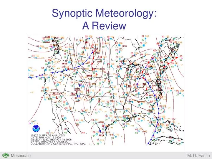
1. Synoptic Meteorology: A Review M. D. Eastin

2. Sun Earth The Role of Mid-Latitude Synoptic Systems The Earth must maintain an Energy (or Heat) Balance! Earth gains energy from the Sun (or warms) via Incoming Shortwave Radiation Earth emits energy to space (or cools) via Outgoing Longwave Radiation M. D. Eastin

3. The Role of Mid-Latitude Synoptic Systems • Maintaining the Global Heat Balance • The Earth cool everywhere via radiation • (the tropics, midlatitudes, and poles) • Due to the Earth’s small tilt with respect • to its axis of rotation, the tropics • received much more energy (heat) • from the Sun than the polar regions • Thus, over time, a strong north-south • gradient in temperature develops • Nature hates strong gradients!!! • The role of mid-latitude synoptic weather • systems is to remove this gradient by transporting (or advecting) warm air poleward and cold air equatorward M. D. Eastin

4. The Role of Mid-Latitude Synoptic Systems • Maintaining the Global Heat Balance • The gradients are continuously removed through the interaction of upper-level waves • in the jet stream with large-scale high and low pressure systems near the surface M. D. Eastin

5. Forces Driving Synoptic-Scale Air Motions • There are five primary forces that govern large-scale atmospheric motions: • Pressure Gradient Force • Gravity • Coriolis Force • Friction • Centrifugal Force • Pressure Gradient Force (PGF) • Pressure is a force per unit area • Air pressure is the weight (mass) of the atmosphere • above a given location • Air pressure is a function of temperature and density • Air pressure decreases with altitude at a decreasing rate • Air always tries to flow down the pressure gradient • from regions of high pressure toward regions of • lower pressure → the pressure gradient force • The pressure gradient force is directly proportional • to the magnitude of the gradient M. D. Eastin

6. Forces Driving Synoptic-Scale Air Motions • Vertical PGF – Gravity – Hydrostatic Balance • The vertical PGF acts to accelerate air upward • Gravity acts to accelerate air parcels downward • (or toward the Earth’s center of mass) • These two forces largely balance each other • This balance is called Hydrostatic Balance • For large-scale (or synoptic-scale) atmospheric • motions vertical accelerations are negligible, • observed vertical motions are weak (1-5 cm/s), • and thus, hydrostatic balance is a valid assumption M. D. Eastin

7. Forces Driving Synoptic-Scale Air Motions • Horizontal PGF – Coriolis Force – Geostrophic Balance • Horizontal PGF: • Acts to accelerate air from regions of high • pressure toward regions of low pressure • Coriolis Force: • Apparent force (Earth is rotating reference frame) • Always acts to accelerate air 90° to the right • of the wind vector in the northern hemisphere • Magnitude is proportional to the wind speed • Geostrophic Balance • When the Coriolis and horizontal PGF are equal • and opposite → Geostrophic Wind • Results in air flow parallel to isobars on height • surfaces and height contours on pressure surfaces • Geostrophic balance is valid assumption for • large-scale atmospheric motions above the • surface (where friction plays a role…) Flow down the pressure gradient M. D. Eastin

8. Forces Driving Synoptic-Scale Air Motions • Horizontal PGF – Coriolis Force – Friction • Horizontal PGF: • Acts to accelerate air from regions of high to low pressure • Coriolis Force: • Always acts to accelerate air 90° to the right (left) • of the wind vector in the northern (southern) hemisphere • Friction • Always acts to slow air parcels down • as they move over rough terrain • (land, trees, buildings, hills, etc.) • Only affects air in the lowest 1-2 km • near the surface • Results in large-scale convergence • (divergence) in association with low (high) • pressure systems near the surface M. D. Eastin

9. Forces Driving Synoptic-Scale Air Motions • Cyclonic Flow • Counter-clockwise flow (N Hemisphere) • Occurs in association with low pressure • systems (called “cyclones”) • Anticyclonic Flow • Clockwise flow (N Hemisphere) • Occurs in association with high pressure • systems (called “anticyclones”) M. D. Eastin

10. Forces Driving Synoptic-Scale Air Motions • Horizontal PGF – Coriolis Force – Centrifugal – Gradient Balance • Horizontal PGF: Accelerates air from regions of high to low pressure • Coriolis Force (Co): Accelerates air 90° to the right of the wind vector • Centrifugal Force (Cf): Results from and applies to curvature in the flow • Accelerates air outward away from the center of rotation • Magnitude is proportional to wind speed • When (Cf + Co) are equal and opposite PGF for flow • around a cyclone → Gradient Wind • The physics involved in gradient balance allow cyclones • to become smaller and more intense than anticyclones (Why?) V Co Co PGF PGF Cf Cf V M. D. Eastin

11. Pressure and Temperature • How does Pressure respond to Temperature Changes? • Increase (decreases) in temperature cause a column of air to expand (contract) • The pressure surfaces move according to this expansion or contraction Warming Upper-level pressure surfaces rise Warming results from: Advection Latent heat release Incoming solar radiation Leads to increases in the 1000-500 mb Thickness Pressures near the surface decrease Cooling Upper-level pressure surfaces sink Cooling results from: Advection Outgoing radiation Leads to decreases in the 1000-500mb Thickness Pressures near the surface increase Altitude 200mb Warming Cooling 850mb L H M. D. Eastin

12. Jet Streams and Jet Streaks • The Midlatitude Jet Stream: • 100-400 miles wide • 500-3000 miles long (non-continuous around the globe) • Winds speeds range 50-200 knots • Located between 200-400 mb (altitude of largest N-S pressure gradient) • Westerly flow in northern hemisphere (Why?) • Moves/Bends/Buckles from day to day in response to large-scale heating / cooling • Play important roles in steering and intensifying/weakening surface highs and lows Jet Stream 250mb Warm Cold Equator North Pole M. D. Eastin

13. Jet Streams and Jet Streaks • The Jet Streaks: • Faster moving pockets of air embedded within the Jet Stream • Produce regions of upper-level divergence and convergence • Have a strong influence on the evolution surface highs and lows • Upper-level divergence will enhance / promote convection and severe weather • Divergence and Convergence • Speed divergence (convergence) results • in a mass decrease (increase), and hence • a surface pressure decrease (increase) • due to air parcel accelerations • Diffluence (Confluence) results in a local • mass and surface pressure decrease • (increase) due to flow in opposite • directions • A net divergence (convergence) often • occurs in the exit (entrance) region, • but this varies from jet streak to jet streak Exit Region Speed Convergence Diffluence Entrance Region Speed Divergence Confluence Jet Streak M. D. Eastin

14. Fronts • Fronts separate different large-scale • air masses (Recall: cP, mT, etc.) • Characterized by large density gradients • whereby the more dense air undercuts • the less dense air • “Local regions” of considerable convective • overturning (i.e. storms) • Fronts are always defined by which way • the more dense (cold and/or dry) air • is moving • Placing Fronts on Weather Maps • Most often defined by strong horizontal • gradients in temperature and/or moisture • Prominent shifts in the wind direction • and elongated “notches” in the pressure • field can help pinpoint a front’s location • Different types of fronts on weather maps • Cold front • Warm front • Stationary front • Occluded front • Surface trough (little or no vertical structure) • Squall line • Dryline • Tropical Wave M. D. Eastin

15. Fronts Placing Fronts on Weather Maps: An Example Fronts and Pressure Temperature Dewpoint Streamlines M. D. Eastin

16. Fronts • Warm Fronts • Slope is gentle and shallow • Move much slower than cold fronts • Warm air overruns the more dense • cold air, rising “slowly” and forming • shallow convection: • Low stratiform clouds • Light precipitation • Precipitation is often well in advance • of the surface frontal boundary M. D. Eastin

17. Fronts • Cold Fronts • Slope is steeper than warm fronts • Move much faster than warm fronts • Warm air is “rapidly” forced over the • cold air, forming deep convection: • Cumulonimbus Clouds • Heavy precipitation • Severe weather • Precipitation is often just ahead of, • along, or just behind the surface • frontal boundary M. D. Eastin

18. Fronts • Occluded Fronts • Occurs when the cold front “catches” • the warm front • The relatively “warm” air (cool air) is • gradually lifted over the cold air • forming shallow convection • Low stratiform clouds • Generally light precipitation • Precipitation is often along the • surface frontal boundary M. D. Eastin

19. The Norwegian Cyclone Model • Provides the basic lifecycle of low pressure • systems in the mid-latitudes • Stage 1: The Stationary Front • Boundary between a cold and war air mass • Air moving parallel to the front • Stage 2: Upper Level Support • A region of upper level divergence moves • over the front and forms an area of surface • low pressure • The circulation around the low starts to bring • cold air south and warm air north • Movement of the air masses forms the cold • and warm fronts Cold Air Warm Air Cold Air Warm Air M. D. Eastin

20. The Norwegian Cyclone Model • Stage 2: Upper-Level Support • Upper-level support is important if the surface • low is to intensify (decrease in pressure) • since friction produces convergence that will • “fill-in” or weaken any low • Support is provided by an eastward moving • synoptic-scale trough (or Rossby wave) in • the jet stream • Divergence, warm air advection, and moist • convection often dominate the region east of • the trough axis (all promote lower surface • pressures) • Surface lows tend to move toward locations • of maximum pressure decrease (which is • often in the area of maximum warm air • advection east of the low) • Similar support is provided for surface highs • in the region east of an upper-level ridge M. D. Eastin

21. The Norwegian Cyclone Model • Stage 3: Organization • Enhanced upper-level divergence continues to • strengthen the surface low • As the low strengthen (pressure drop), the fronts • become better organized • The stronger winds around a stronger low allows • more cold and warm air advection to occur • Stage 4: Maturity • The upper-level low begins to catch the surface • low and the divergence wanes • The surface low reaches its lowest pressure • The cold front (moving faster) “catches” the warm • front, forming an occluded front • In the occluded front, the cold air undercuts the • “cooler air” ahead of the warm front, so lifting still • occurs but it is less vigorous (stratiform clouds • and precipitation) Cold Air Cool Air Warm Air Cool Air Cold Air Warm Air M. D. Eastin

22. The Norwegian Cyclone Model • Stage 4: Maturity • Once the occlusion forms, the low pressure is • separated from the warm air mass and thus the • warm air advection • The motion of the surface system slows • The upper-level low “catches” the surface low • and is now located directly above (the system • is now “stacked”) • What happens next? • Stage 5: Dissipation • With the upper-level low and its associated • convergence directly above the surface low, • the surface low begins to “fill-in” and • eventually dissipates • The remains of the warm and cold front will form • a stationary boundary and await the next • upper-level trough…. Cold Air Warm Air Cold Air Warm Air M. D. Eastin

23. Thermodynamic Concepts and Stability Basic Definitions of Meteorological Quantities: Vapor Pressure (e):Partial pressure of water vapor in the air Mixing Ratio (w):Mass of vapor to the mass of dry air Saturation Mixing Ratio (ws): Maximum vapor mass for a given temperature and pressure Relative Humidity: 100 x (mixing ratio / saturation mixing ratio) Specific Humidity (q): Mass of vapor to the mass of moist air Dewpoint Temperature (Td): Temperature of a air parcel if cooled to saturation at constant pressure Virtual Temperature (Tv): Temperature a dry air parcel would have if its density equaled that of a moist air parcel at the same temperature and pressure M. D. Eastin

24. Thermodynamic Concepts and Stability Basic Definitions of Meteorological Quantities: Potential Temperature (θ): Temperature of air if brought dry-adiabatically to 1000 mb Wet-bulb Temperature (Tw): Equilibrium temperature whereby the latent heat loss (or cooling) induced by evaporation is balanced by the flow of heat (warming) from the surrounding warmer air Equivalent Temperature (Te): Temperature an air parcel would have if all of its latent heat was released Equivalent Potential Temperature (θe): Temperature of a parcel if all moisture is condensed out (latent heat release) and the parcel is brought dry-adiabatically to 1000 mb M. D. Eastin

25. Thermodynamic Concepts and Stability Adiabatic Processes: Parcels of air expand and cool, or compress and warm, with no exchange of heat with the environment A reversible process Dry Adiabatic Process: If the parcel does not saturate, then the warming or cooling occurs at the dry adiabatic lapse rate, which is constant in our atmosphere (~0.1ºC/mb or ~10ºC/km in the vertical) Moist Adiabatic Process: If the parcel saturates, condensation and latent heat release occurs, and the parcel cools at the slower moist adiabatic lapse rate, which varies with temperature and moisture (but averages ~0.06ºC/mb or ~6.5ºC/km in the vertical) Pseudo-Adiabatic Process: If an air parcel saturates, condenses water, and the water is removed from the parcel (i.e., rainfall), the parcel will still cool at the moist adiabatic lapse rate, but the process is no longer reversible (loss of heat energy in the liquid water) M. D. Eastin

26. Thermodynamic Concepts and Stability • Five Types of Thermal Stability in the Atmosphere: • 1. Absolute Instability: • Environmental (or observed) lapse rate is greater • than the dry adiabatic lapse rate • Air parcels will spontaneously accelerate (via dry • convection) to remove the “super-adiabatic” layer • 2. Dry Neutral Stability: • Environmental and dry adiabatic lapse rates are equal • Often observed in the boundary layer (“mixed” layer) z Moist Dry Env T z Env Moist Dry T M. D. Eastin

27. Thermodynamic Concepts and Stability • Five Types of Thermal Stability in the Atmosphere: • 3. Conditional Instability: • Environmental (or observed) lapse rate is less than • the dry adiabatic lapse rate but greater than the • moist-adiabatic lapse rate • Air parcels will spontaneously accelerate (via moist • convection) once the parcel becomes saturated • Any vertical displacement of an unsaturated parcel • will result in an acceleration back toward its original • location. • Most common state of the atmosphere z Moist Dry Env T M. D. Eastin

28. Thermodynamic Concepts and Stability • Five Types of Thermal Stability in the Atmosphere: • 4. Moist Neutral Stability: • Environmental lapse rate is equal to the moist • adiabatic lapse rate • Often observed in the tropical cyclones or the • center of large thunderstorms • 5. Absolute Stability: • Environmental lapse rate is less than both the dry and • moist adiabatic lapse rates • Temperature inversions are an example • Any vertical displacement of an air parcel will result in • an acceleration back toward its original location z Env Moist Dry T z Moist Dry Env T M. D. Eastin

29. Skew-T Log-P Diagrams A convenient way to: Examine the vertical structure of the atmosphere Determine unreported meteorological quantities Assess air parcel stability M. D. Eastin

30. Skew-T Log-P Diagrams Basic Definitions of Meteorological Quantities: Lifting Condensation Level (LCL): Altitude whereby a parcel becomes saturated by lifting dry-adiabatically Mixing Condensation level (MCL): Altitude whereby a parcel with the mean properties of a layer (a mixed layer) becomes saturated by lifting dry-adiabatically Convective Condensation Level (CCL): Altitude whereby a parcel, if heated sufficiently, will rise dry-adiabatically until it becomes saturated Convective Temperature (Tc): Temperature that must be reached for a parcel to rise to its CCL Level of Free Convection (LFC): Altitude whereby a parcel lifted dry-adiabatically to saturation, and then moist adiabatically, first becomes warmer than the surrounding air Equilibrium Level (EL): Altitude where the temperature of a buoyant air parcel (above an LFC) becomes equal to the surrounding air temperature M. D. Eastin

31. Skew-T Log-P Diagrams Basic Definitions of Meteorological Quantities: Positive Area (or CAPE): Area between the environmental sounding and the moist adiabat of the parcel at altitudes between the LFC and the EL Proportional to the amount of energy the parcel gains from the environment. Large values often lead to deep convection with strong updrafts Negative Area (or CIN): Area between the environmental sounding and the moist adiabat of the parcel at altitudes between the condensation level (either LCL, MCL, or CCL) and the LFC Proportional to the amount of energy need to move to parcel Large values can inhibit deep convection Wet-Bulb Zero: Altitude where the wet-bulb temperature first reaches 0ºC This is the altitude where ice (snow and hail) begins to melt M. D. Eastin

32. Skew-T Log-P Diagrams M. D. Eastin

33. Skew-T Log-P Diagrams M. D. Eastin

34. Skew-T Log-P Diagrams M. D. Eastin

35. Skew-T Log-P Diagrams M. D. Eastin

36. Skew-T Log-P Diagrams M. D. Eastin

37. Skew-T Log-P Diagrams Temperature (oC) -30 -40 -20 -50 -60 200 Equilibrium Level -10 300 0 Positive Area Pressure (mb) 400 10 20 500 30 Level of Free Convection 600 40 700 LCL 800 900 Td T 1000 M. D. Eastin

38. Skew-T Log-P Diagrams Temperature (oC) -30 -40 -20 -50 -60 200 Equilibrium Level -10 300 0 Pressure (mb) 400 10 20 500 30 Level of Free Convection 600 40 700 Negative Area LCL 800 900 Td T 1000 M. D. Eastin

39. Skew-T Log-P Diagrams • Stability Indices: • Help the forecaster evaluate the likelihood and type of thunderstorms and severe weather • from an individual sounding • Each index has advantages and disadvantages, but all are relatively easy to compute • Showalter Index (SI) • Lifted Index (LI) • K-Index (KI) • Total Totals (TT) • SWEAT Index • Convective Available Potential Energy (CAPE) • Convective Inhibition (CIN) • Bulk Richardson Number (BRN) • Environmental Helicity • Storm-relative Helicity • Note: Detailed descriptions of how to calculate the first five indices and their resulting • index values associated with thunderstorm potential are in the Skew-T manuals • available on the course website M. D. Eastin

40. Synoptic Meteorology: The “Stage” for Mesoscale Events • Summary of Concepts and Tools: • Role of Mid-Latitude Weather Systems • Five Forces Driving Synoptic Scale Air Motions • Relationship between Pressure and Temperature • Jet Streams and Jet Streaks • Fronts (Cold, Warm, Occluded) • Norwegian Cyclone Model • Thermodynamic Concepts • Five Types of Stability • Skew-T Log-P Diagrams M. D. Eastin