Multivariate Machine Learning Methods: New Developments and Applications in HEP

1. Multivariate Machine Learning Methods: New Developments and Applications in HEP Pushpa Bhat Fermilab August 6, 2015

2. No turning back! • Over the past 25 years, Multivariate analysis (MVA) methods have gained gradual acceptance in HEP. • In fact, they are now “state of the art” • Some of the most important physics results in HEP, in the past two decades, have come from the use MVA methods. • In 1990’s, I’d have on my title slide “We are riding the wave of the future” • That future is here, and MVA methods are here to stay!

3. Important Physics Results • From top quark to the Higgs … and many smart applications in object ID, energy corrections, as well • Top-antitop event selection optimization – 1990-95 (D0) • Top quark mass measurement -- 1996-97 • Top cross section measurements in all channels (1995 - ) • Top observation in the all-jets channel (D0) (1999) • New particle/physics searches (1997 - ) • Observation of single top quark production (2009) • Evidence for Higgs bb at the Tevatron (2012) • Higgs Discovery at the LHC in2012

4. MVA for Top quark in the mid-90’s DØ Lepton+jets e+jetscut optimization for cross section measurement The Discriminants Top Quark Mass Measurement LB: Low-bias maximum likelihood NN: Neural Networks Observation in all-jets channel mt = 173.3 ± 5.6(stat.) ± 6.2 (syst.) GeV/c2 Fit performed in 2-D: (DLB/NN, mfit)

5. MVA use in Higgs Discovery • MVA used in every possible analysis aspect • Electrons/photons ID • MVA regression for EM cluster energy corrections • Vertex identification (diphotons) • b-tagging • S/B discrimination in all channels • γγ, ZZ4l, (WW, bb, ττ)

6. Broad Categories of Analysis Tasks • Classification • Object ID with high efficiency and low fake rates • Identification of electrons, photons, taus, b-quark jets, .. • signal/background discrimination • Parameter Estimation • Measurement of quantities; observables  parameters • Function fitting • Energy correction functions, tag-rate functions, … Mathematically, all of these are Functional Approximation problems.

7. Classification • In classification, the function to be approximated is where SandBdenote signal and background, respectively. • In practice, it is sufficient to approximate the discriminant because D(x) and p(S|x) are related one-to-one: where A = p(S) / p(B) is the prior signal to background ratio

8. Multivariate Methods A list of popular methods • Random Grid Search • Linear Discriminants • Quadratic Discriminants • Support Vector Machines • Naïve Bayes (Likelihood Discriminant) • Kernel Density Estimation • Neural Networks • Bayesian Neural Networks • Decision Trees • Random Forests • Genetic Algorithms

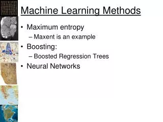
9. Machine Learning • Paradigm for automated learning from data, using computer algorithms • Has origins in the pursuit of artificial intelligence starting ~1960 • Requiring little a priori information about the function to be learned • A method that can approximate a continuous non-linear function to arbitrary accuracy is called a universal approximator • e.g. Neural Networks

10. Machine Learning Approaches • Supervised Learning • Supervised learning with a training data set containing feature variables (inputs) and target to be learned: {y,x} • Unsupervised Learning • No targets provided during training. • Algorithm finds associations among inputs. • Reinforcement Learning • Correct outputs are rewarded, incorrect ones penalized.

11. “Rectangular” Cuts Regular Grid search Signal eff. Vs bkgd. eff ROC RGS can serve as a benchmark for comparisons of efficacy of variables, variable combinations, and classifiers Random Grid search (RGS) Find “best” cuts H.B.Prosper, P.Bhat, et al. CHEP’95

12. Neural NetworksThe Bayesian Connection • The output of a neural network can approximate the Bayesian posterior probability p(s|x): where Train to minimize Flexible, non-linear model

13. RGS vs NN • Random Grid Search for “cut” optimization • The best “cut-based” analysis you can do! • Notice that NN can provide significant gains even in this simple 2D analysis, at lower backgrounds which is the region of interest MVA Simple cuts A simple illustration of MVA PB, Annu. Rev. Nucl. Part. Sci. 2011, 61:281-309. Simple cuts

14. NN/MVA vs Bayes NN (or any other fully multivariate technique) can provide discrimination close to the Bayes limit PB, Annu. Rev. . 61 (2011) PB, Annu. Rev. . 61 (2011) P.Bhat, Annu. Rev. Nucl. Part. Sci. 61, 281-309 (2011)

15. Bayesian Neural Networks • Instead of attempting to find a single “best” network, i.e., a single “best” set of network parameters (weights), with Bayesian training we get a posterior density for the network weights, p(w| T), T Training data • The idea here is to assign a probability density to each point win the parameter space of the neural network. Then one takes a weighted average over all points, i.e., over all possible networks. • Advantages: • Less likely to be affected by “over training” • No need to limit the number of hidden nodes • Good results with small training sample P.C. Bhat, H.B. Prosper Phystat 2005, Oxford

16. Boosted Decision Tree (BDT) • A Decision Tree (DT) recursively partitions feature space into regions or bins with edges aligned with the axes of the feature space. • Aresponse value is attached to each bin, • D(x) = s/(s+b) • Boosting: Make a sequence of M classifiers (DTs) that successively handle “harder” events and take a weighted average  BDT

17. An Example PB, Annu. Rev. . 61 (2011) PB, Annu. Rev. . 61 (2011) PB, Annu. Rev. . 61 (2011) P.Bhat, Annu. Rev. Nucl. Part. Sci. 61, 281-309 (2011)

18. What method is best? • The “no free lunch” theorem tells you that there is no one method that is superior to all others for all problems. • In general, one can expect Bayesian neural networks (BNN), Boosted decision trees (BDT) and random forests (RF) to provide excellent performance over a wide range of problems. • BDT is popular because of robustness, noise resistance (and psychological comfort!)

19. The Buzz about Deep Learning • A lot of excitement about “Deep Learning” Neural Networks (DNN) in the Machine Learning community • Spreading to other areas! • Some studies already in HEP! • Multiple non-linear hidden layers to learn very complicated input-output relationships • Huge benefits in applications in computer vision (image processing/ID), speech recognition and language processing

20. Deep Learning NN • Use raw data inputs instead of derived “intelligent” variables (or use both) • Pre-processing or feature extraction in the DNN • Pre-train initial hidden layers with unsupervised learning • Multi-scale Feature Learning • Each high-level layer learns increasingly higher-level features in the data • Final learning better than shallow networks, particularly when inputs are unprocessed raw variables! • However, need a lot of processing power (implement in GPUs, time (and training examples)

21. Deep Learning Single hidden layer NN “Dropout” algorithm to avoid overfitting (pruning) Multiple hidden layer NN

22. Deep Neural Networks for HEP • Baldi, Padowski, WhitesonarXiv:1402.4735v2 • Studied two benchmark processes • Charged Higgs vsttbar events • SUSY: Charginopairs vs WW events into dilepton+MET final state Significant improvement in Higgs case, not so dramatic in case of SUSY SUSY SUSY Higgs Higgs Exotic Higgs SUSY Study

23. Unsupervised Learning • The most common approach is to find clusters or hidden patterns or groupings in data • Common and useful methods • K-Means clustering • Gaussian mixture models • Self-organizing maps (SOM) • We have not tapped these methods for identifying unknown components in data, unsupervised classification, for exploratory data analysis • Could be useful in applications for topological pattern recognition • Use in Jet-substructure, boosted jet ID http://chem-eng.utoronto.ca/~datamining/Presentations/SOM.pdf

24. Challenges in LHC Run 2 and beyond • Challenges: • Pile-Up mitigation! • <PU>~40 in Run2 • Associating tracks to correct vertices • Correcting jet energies, MET, suppressing fake “pileup” jets, • Lepton and photon isolation • Boosted Objects • Complicates Object ID • W, Z, Higgs, top taggers! • Provides new opportunities • Use jet substructure • High energy Lepton ID • Signals of BSM could be very small • Small MET in SUSY signatures (compressed, stealth,… ) • Need new algorithms, approaches for reco and analysis • New ideas in triggering and data acquisition

25. Summary • Multivariate methods brought a paradigm shift in HEP analysis ~20 years ago. Now they are state of the art. • Applications of new ideas/algorithms such as deep learning should be explored, but the resources involved may not justify the use in every case. • Revived emphasis on unsupervised learning is good and should be exploited in HEP. • Well established techniques of the past – single hidden layer neural networks, Bayesian neural networks, Boosted Decision Trees should continue to be the ubiquitous general purpose MVA methods.

26. Extra slides

27. Optimal Discrimination • More dimensions can help! • One dimensional distributions are marginalized distributions of multivariate density. • f(x1)=g(x1,x2,x3, .. )dx2dx3.. xcut  Minimize the total misclassification error Significance level 1-: Power

28. Minimizing Loss of Information.. And Risk • General Approach to functional approximation • Minimize Loss function: • It is more robust to minimize average loss over all predictions or a cost (or error) function: • There are many approaches/methods A common Risk function Constraint

29. Calculating the Discriminant • Density estimation, in principle, is simple and straightforward. • Histogramming: • Histogram data in M bins in each of the d feature variables Md bins  Curse Of Dimensionality • In high dimensions, we would need a huge number of data points or most of the bins would be empty leading to an estimated density of zero. • But, the variables are generally correlated and hence tend to be restricted to a sub-space Therefore, Intrinsic Dimensionality << d • There are more effective methods for density estimation