Applying Constraint Satisfaction Techniques to AI Planning Problems

1. Applying Constraint Satisfaction Techniques to AI Planning Problems Daniel Buettner Constraint Systems Laboratory Department of Computer Science and Engineering University of Nebraska-Lincoln Under the supervision of Dr. Berthe Y. Choueiry

2. Outline • Background • The GP-CSP planning system • Exploiting partial interchangeability • Investigating decomposition • Maintaining Arc Consistency (MAC) • Conclusion

3. Questions addressed • Are CSP techniques suitable for solving AI planning problems? • Yes! • Is Dynamic Neighborhood Partial Interchangeability (DNPI) effective in the context of CSP formulations of AI planning problems? • Not with the CSP formulation that we have studied.

4. Questions addressed… • Is there an effective conjunctive decomposition for planning problems formulated as CSPs? • Not with the CSP formulation that we have studied. • Is Maintaining Arc Consistency (MAC) an effective algorithm for finding solutions to CSP formulations of AI planning problems? • Yes! • How does MAC perform with various variable orderings? • MAC performs well on a wide range of variable orderings.

5. Contributions • We have found a variable pruning method for our CSP representation • We have shown that DNPI cannot work with our CSP representation • We provide an iterative implementation of MAC • We identify some dynamic variable ordering schemes for MAC that work well on AI planning problems

6. Background

7. Background • Introduction to AI planning • Introduction to Constraint Satisfaction • Introduction to the GP-CSP planning system

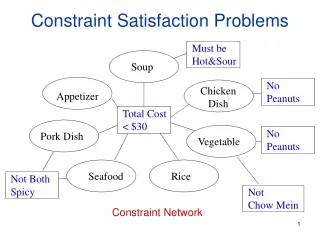
8. AI planning • A planning problem is one in which an agent capable of sensing and of performing some actions finds itself in a world, needing to achieve certain goals • A solution to a planning problem is an ordered sequence of actions that, when carried out, will achieve the desired goals • An example will help illustrate this.

9. Planning example • A simple example of such a problem is one in which two men, Jason and Alex, are initially in London with Jason wishing to travel to New York and Alex wishing to travel to Paris. There are two rockets in London, each capable of carrying one or more persons and making a single flight. • The available actions allow one to: • load a person into a rocket • fly a rocket from one city to another • unload a person from a rocket.

10. Planning example… • One solution to this problem is the following sequence of actions: • Load Jason into rocket 1 • Load Alex into rocket 2 • Fly rocket 1 to New York • Fly rocket 2 to Paris • Unload Jason from rocket 1 • Unload Alex from rocket 2

11. AI planning… • A planning problem should specify: • A description of the world's initial state (as a set of facts) • A description of the agent's goal (as a set of facts) • A description of the possible actions that can be carried out to affect the state of the world • Planning systems read domain and problem descriptions in a standard language called PDDL

12. Classical AI planning • Several simplifying assumptions are made in classical AI planning: • All actions require a single, uniform, unit of time to execute • Actions will be successful and produce their expected results • The agent knows the initial state of the world, as well as the impact of its own actions on the state of the world • The only change in the world is the result of the agent's own actions

13. GraphPlan • Planning system introduced in 1995 by Blum and Furst • Today’s fast planning systems use stochastic techniques and sacrifice guarantees of optimality; however, planning systems that guarantee optimality in time steps are still based on the ideas of GraphPlan

14. GraphPlan… • GraphPlan finds solutions to planning problems by constructing a planning graph level-by-level, and searching for valid plans within that graph • Planning graphs consist of alternating layers of facts and actions

15. The planning graph • When a planning graph is first created, it simply contains a fact layer made up of the initial conditions that specify the initial state of the planning problem

16. The planning graph… • Planning graphs are extended by finding all actions whose prerequisites are satisfied at the most recent fact level and adding these actions in the next layer of the graph • The effects of these actions form the next fact layer • a so-called noop action exists that can take any fact as a prerequisite with that same fact as the action's only effect

17. GraphPlan mutexes • GraphPlan discovers binary mutual exclusion (mutex) relationships between actions and facts • Actions are mutex when: • The effect of one action is the negation of another action's effect • One action deletes the precondition of another • The actions have preconditions that are marked as mutex

18. GraphPlan mutexes… • Facts are mutex when: • One fact is the negation of the other • All actions supporting the facts are pairwise mutex • Mutex relationships are specific to levels in the planning graph; a pair of facts that are mutex in one level of the planning graph may not be mutex at later levels

19. Plan extraction • Plan extraction is first attempted when all of the goals are present in the highest fact layer and are non-mutex • Plans are extracted via a simple backtracking search, starting with the highest fact layer • If no plan is found, the planning graph is extended and GraphPlan attempts plan extraction on this new planning graph

20. Plan extraction… • Graphplan first searches for a solution at the earliest possible point that a plan could exist • It incrementally extends the planning graph if no solution is found • Thus, GraphPlan finds the plan that uses the fewest time steps and is therefore optimal in this respect • However, GraphPlan allows multiple actions to occur at each time step and so it cannot guarantee optimality in the total number of actions in the plan

21. GraphPlan concluded • Our work is based upon the ideas of GraphPlan • We convert the planning graph to a Constraint Satisfaction Problem (CSP) and extract solutions by solving the CSP • Next: introduction to Constraint Satisfaction

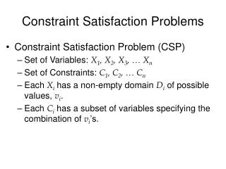
22. Constraint satisfaction • Constraint satisfaction is a general method of problem formulation in which the goal is to find values for variables such that these values do not violate any constraints that hold between the variables

23. Definitions • A Constraint Satisfaction Problem (CSP) involves: • A set of variables {V1, V2, … , Vn} • Each variable Vi has an associated domain Diwhich specifies the possible values of the variable • Finally, there exists a set of constraints between the variables • a constraint is a relation that restricts the values that variables involved in the constraint may simultaneously hold

24. CSP example • D1={R, G, B},D2={R, G}, and D3={R, G, B} • The constraints all require that certain variables not assume the same value • A CSP is solved when a value is found for each variable such that no constraints are violated • V1 := R, V2 := G, V3 := B

25. Solution extraction • While looking for solutions, the variables are considered in some order • As a partial solution is constructed, past variables are those that have been instantiated, while future variables are those that have not yet had a value assigned to them

26. Solution extraction… • One of the simplest systematic methods of finding a solution to a CSP is a depth first backtracking search • This search proceeds by starting with the first variable and assigning it the first value in that variable's domain • It then moves to the next variable and checks the first value in that variable's domain against the previously assigned variable; if there is no problem it moves on to the next variable, otherwise it tries the next value in the current variable's domain

27. Forward checking • Forward checking (FC) is a more intelligent method for finding a solution to a CSP • A look-ahead scheme in which consistency with future variables is ensured, removing the need to check against previously assigned variables • When a variable is assigned a value, that value is used to filter the domains of future variables • By always checking forward, we eliminate the need to reconsider past variables • Next: GP-CSP

28. The GP-CSP planning system

29. GP-CSP • Our work extends a planning system called GP-CSP (Do and Kambhampati 2001) • GP-CSP unifies the traditional GraphPlan method for planning with CSP methods for solution extraction • GraphPlan's plan extension is unchanged while the normal backtracking search is replaced with a CSP solver

30. GP-CSP… • The architecture of the GP-CSP system

31. CSP formulation • CSP variables represent facts • The variable domains are the actions supporting these facts • Each variable has an extra value called NOTHING added to it, which allows a fact to be left with no support • The constraints between variables enforce action and fact mutexes, as well as activity constraints • The transformation from GraphPlan’s planning graph to a CSP of this type is straight forward and is carried out automatically by GP-CSP

32. Our changes to GP-CSP • We have replaced their general GAC solver with a strictly binary solver which is extended to perform: • Dynamic symmetry detection • Decomposition • Maintaining Arc Consistency (MAC) • We have our own representation of the CSP formulation just described which takes advantage of the object orientation of C++

33. Preprocessing • We have discovered a preprocessing step that can reduce certain variables to a single value • These variables have only the actions noop and NOTHING in their domains, and they are only constrained to act as prerequisites for other actions • Such variables correspond to facts that encode typing information • This typing information is necessary during creation of the planning graph, but is no longer needed during solution extraction and can then be ignored

34. Preprocessing results

35. GP-CSP concluded • We tried several static variable orderings in conjunction with Forward Checking • The default ordering obtained by moving backwards in the planning graph from highest layer to lowest was the only effective ordering • Next: Partial interchangeability

36. Exploiting partial interchangeability

37. Exploiting partial interchangeability • Interchangeability amongst the values of a variable in a CSP is a term used to describe an equivalence that exists between these values • The idea is that if values d1 and d2 for variable Vi are found to be interchangeable, then any solution to the CSP with Vi taking the value d1 will remain a solution if the value is changed to d2

38. Interchangeability is good • Interchangeable values: • help to create more robust solutions since failures can potentially be repaired by simply substituting values instead of resolving • can help to reduce the search space, by allowing us to replace the interchangeable (or bundled) values with a single meta-value

39. DNPI • Full interchangeability is expensive to compute • Partial interchangeability finds a subset of interchangeable values with lower overhead • Dynamic neighborhood partial interchangeability (DNPI) requires the same computations as FC with some additional bookkeeping

40. DNPI… • How does it work? • When a variable is first considered, forward checking is performed with each of that variable’s values • A structure called the Joint Discrimination Tree captures this information and bundles values that have the exact same impact on future variables • Sets of bundled values are replaced in the variable's domain with a single meta-value, thus reducing the search space

41. Application to planning • There are many situations in which planning problems exhibit what seem to be symmetric actions • In the gripper domain a robot with a right and left arm needs to move a set of balls from one room to another • It does not matter whether the left arm or right arm moves a ball • Each robot arm cares little about the distinction between the different balls

42. Application to planning… • Unfortunately, DNPI is unable to take advantage of this symmetry • Recall that values are interchangeable only when they have the same impact on future variables • However, in our CSP formulation, different values do not share the same neighborhood • Each value represents an action, and actions do not share the same preconditions, effects, and mutexes unless they are identical actions

43. DNPI concluded • The explicit naming of objects in PDDL prevents DNPI from bundling values in our CSP representation • An instantiation of an action must refer to particular facts as preconditions and effects, so no two actions refer to the same set of facts unless the actions are identical • Next: Decomposition

44. Investigating decomposition

45. Investigating decomposition • It is sometimes possible to more efficiently solve a problem by decomposing that problem into a set of independent subproblems • Each subproblem can be independently solved, and those solutions can be combined to form a solution to the original problem

46. Tree clustering • We investigated the tree clustering algorithm of Dechter and Pearl • This is a method of restructuring a CSP to make solution extraction less costly • The constraint graphs that are created by converting a planning problem to our CSP representation exhibit structure that makes decomposition quite simple

47. Tree clustering…

48. Decomposition • We can start at the highest level in the planning graph and form a new CSP with the variables one layer lower • Only the constraints between this subset of variables are kept • We can again form a new CSP, this time using the next lowest layer • We continue in this way until we reach the layer of initial conditions • An n layer planning graph will be decomposed into n-1 CSPs

49. Results • Ideally, each CSP can now be solved separately, and their individual solutions will be combined to form a solution to the original problem • However, this decomposition makes things worse • A planning graph is a compact representation of many planning problems • The lower subproblems do not have access to goal information and will have, as solutions, parts of valid plans that have nothing to do with the problem we are solving

50. Results… • The only way tree clustering can be made to perform well is to consider the subproblems from the top down, propagating goal information backwards • This corresponds to using forward checking with the default GraphPlan variable ordering • Thus tree clustering did not improve our ability to find a solution, but it does explain why we had such good results with forward checking and GraphPlan’s default ordering • Next: MAC