Download
1 / 12
120 likes | 204 Views
Package Transportation Scheduling . Albert Lee Robert Z. Lee. Problem Summary. UPS – Scheduling of deliveries, set number of trucks (machines), a set list of locations (nodes), and trying to optimize routes with consideration to stochastic nature of traffic

E N D
Package Transportation Scheduling Albert Lee Robert Z. Lee
Problem Summary • UPS – Scheduling of deliveries, set number of trucks (machines), a set list of locations (nodes), and trying to optimize routes with consideration to stochastic nature of traffic • To simplify, we approach the problem with one delivery truck and one depot, making deliveries to multiple delivery locations with stochastic travel time. • Difficulty: What is ideal, the path with lowest mean travel time or with lowest variance? • Difficulty: Stochastic nature of travel times means that optimal path is constantly changing. What is optimal one second may not be optimal the next.
Proposed Solution • Stochastic dynamic traveling salesman problem with time windows (SDTSPTW). • Assumption of travel time between nodes being approximated by normal distribution • If delivery window is too small for a feasible solution with one truck, more trucks need to be added • Heuristic algorithm using n-path relaxation of TSP and convolution-propagation approach
N-path Relaxation and Loop Elimination • For a traveling salesman problem to minimize the total transportation cost for n customers (i.e., nodes), find a lower bound of the objective function by solving shortest-path problems of at most n links. • Partial route (l-path) is a route built by adding links – it is an l-path at node j if the route of l links ends at node j • To eliminate links that loop (i-j-i) we will track both the best and 2nd best routes of any l-path of any node, and if the best route is i-j-I, then the 2nd best is used.
Convolution-Propagation Approach • Used as a mechanism to predict the arrival time of the vehicle at a node on the specified delivery route. • CPA provides the normal distribution (mean, variance) of the arrival time at the node, which is helpful as we are looking at a stochastic model
Model • N := {n nodes} and A := {m links} s.t. graph G = (N,A) is connected. • Node 0∈N denotes the depot from which the delivery truck originates • Truck begins from Node 0 and must visit all other n-1 nodes, then return to Node 0. • For Node i ∈ N, there exists some time window restriction in which the truck must arrive within in order to successfully make the delivery. • Delivery processing time is denoted as Si (service time at node i), where Si ~ N(Vi, θi2)
Model (cont’d) • Time horizon [0, ∞] split into T segments s.t. I0 (=0) < I1 <…<IT-1<IT = ∞. • Travel time D of the truck between nodes is time dependent (traffic varies depending on the time) • if the route starts in [It−1, It), t = 1, …, T, the travel time D ~ N(δ + ρt,σt2), where δ is the constant least possible (free flow) travel time and ρt is the random delay time of starting within the tth time interval.
Elimination of Routes • Must check if subroutes satisfy all time windows of each node by checking known distribution arrival times Yi against some variable ϒ representing the maximum allowable tardiness probability, such that we reject the route if P (Yi ≥ ui) > ϒ • In the case of two routes arriving at one node, we consider if both the mean and variance of the arrival time of route A (B) are smaller than the corresponding values of route B (A), route A (B) is more efficient than route B (A); the inefficient route is discarded. If the mean of one route is smaller but the variance is larger than the other route, the two routes do not dominate each other; both are efficient and both are kept.
Equation References: • Equation 6: • Equation 7:
Equation References Cont’d: • Equation 8:
Sample Network Illustration Starting at node 0, travelling to one of 5 nodes in step 1, from there travelling to one of remaining 4 nodes in step 2, so on and so forth until all nodes have been visited and return to node 0. TSP transformed to SP (shortest path)