Download
1 / 54
540 likes | 545 Views
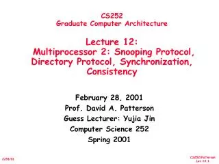
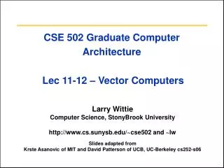
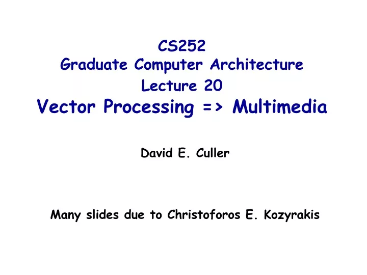
CS252 Graduate Computer Architecture Lecture 20 Vector Processing => Multimedia. David E. Culler Many slides due to Christoforos E. Kozyrakis. VECTOR (N operations). SCALAR (1 operation). v2. v1. r2. r1. +. +. r3. v3. vector length. add r3, r1, r2. vadd.vv v3, v1, v2.

E N D
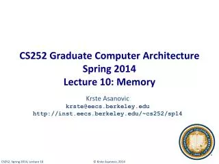
CS252Graduate Computer ArchitectureLecture 20Vector Processing => Multimedia David E. Culler Many slides due to Christoforos E. Kozyrakis
VECTOR (N operations) SCALAR (1 operation) v2 v1 r2 r1 + + r3 v3 vector length add r3, r1, r2 vadd.vv v3, v1, v2 Vector Processors • Initially developed for super-computing applications, today important for multimedia. • Vector processors have high-level operations that work on linear arrays of numbers: "vectors"
Properties of Vector Processors • Single vector instruction implies lots of work (loop) • Fewer instruction fetches • Each result independent of previous result • Multiple operations can be executed in parallel • Simpler design, high clock rate • Compiler (programmer) ensures no dependencies • Reduces branches and branch problems in pipelines • Vector instructions access memory with known pattern • Effective prefetching • Amortize memory latency of over large number of elements • Can exploit a high bandwidth memory system • No (data) caches required!
Styles of Vector Architectures • Memory-memory vector processors • All vector operations are memory to memory • Vector-register processors • All vector operations between vector registers (except vector load and store) • Vector equivalent of load-store architectures • Includes all vector machines since late 1980s • We assume vector-register for rest of the lecture
Historical Perspective • Mid-60s fear perf. stagnates • SIMD processor arrays actively developed during late 60’s – mid 70’s • bit-parallel machines for image processing • pepe, staran, mpp • word-parallel for scientific • Illiac IV • Cray develops fast scalar • CDC 6600, 7600 • CDC bets of vectors with Star-100 • Amdahl argues against vector
Cray-1 Breakthrough • Fast, simple scalar processor • 80 MHz! • single-phase, latches • Exquisite electrical and mechanical design • Semiconductor memory • Vector register concept • vast simplification of instruction set • reduced necc. memory bandwidth • Tight integration of vector and scalar • Piggy-back off 7600 stacklib • Later vectorizing compilers developed • Owned high-performance computing for a decade • what happened then? • VLIW competition
Components of a Vector Processor • Scalar CPU: registers, datapaths, instruction fetch logic • Vector register • Fixed length memory bank holding a single vector • Typically 8-32 vector registers, each holding 1 to 8 Kbits • Has at least 2 read and 1 write ports • MM: Can be viewed as array of 64b, 32b, 16b, or 8b elements • Vector functional units (FUs) • Fully pipelined, start new operation every clock • Typically 2 to 8 FUs: integer and FP • Multiple datapaths (pipelines) used for each unit to process multiple elements per cycle • Vector load-store units (LSUs) • Fully pipelined unit to load or store a vector • Multiple elements fetched/stored per cycle • May have multiple LSUs • Cross-bar to connect FUs , LSUs, registers
Cray-1 Block Diagram • Simple 16-bit RR instr • 32-bit with immed • Natural combinations of scalar and vector • Scalar bit-vectors match vector length • Gather/scatter M-R • Cond. merge
Basic Vector Instructions Instr. OperandsOperationComment VADD.VVV1,V2,V3 V1=V2+V3 vector + vector VADD.SVV1,R0,V2 V1=R0+V2 scalar + vector VMUL.VV V1,V2,V3 V1=V2xV3 vector x vector VMUL.SV V1,R0,V2 V1=R0xV2 scalar x vector VLD V1,R1 V1=M[R1..R1+63] load, stride=1 VLDS V1,R1,R2 V1=M[R1..R1+63*R2] load, stride=R2 VLDX V1,R1,V2 V1=M[R1+V2i,i=0..63] indexed("gather") VST V1,R1 M[R1..R1+63]=V1 store, stride=1 VSTS V1,R1,R2 V1=M[R1..R1+63*R2] store, stride=R2 VSTX V1,R1,V2 V1=M[R1+V2i,i=0..63] indexed(“scatter") + all the regular scalar instructions (RISC style)…
Vector Memory Operations • Load/store operations move groups of data between registers and memory • Three types of addressing • Unit stride • Fastest • Non-unit(constant) stride • Indexed (gather-scatter) • Vector equivalent of register indirect • Good for sparse arrays of data • Increases number of programs that vectorize • compress/expand variant also • Support for various combinations of data widths in memory • {.L,.W,.H.,.B} x {64b, 32b, 16b, 8b}
64 element SAXPY: scalar LD R0,a ADDI R4,Rx,#512 loop: LD R2, 0(Rx) MULTD R2,R0,R2 LD R4, 0(Ry) ADDD R4,R2,R4 SD R4, 0(Ry) ADDI Rx,Rx,#8 ADDI Ry,Ry,#8 SUB R20,R4,Rx BNZ R20,loop 64 element SAXPY: vector LD R0,a #load scalar a VLD V1,Rx #load vector X VMUL.SV V2,R0,V1 #vector mult VLD V3,Ry #load vector Y VADD.VV V4,V2,V3 #vector add VST Ry,V4 #store vector Y Vector Code Example Y[0:63] = Y[0:653] + a*X[0:63]
Vector Length • A vector register can hold some maximum number of elements for each data width (maximum vector length or MVL) • What to do when the application vector length is not exactly MVL? • Vector-length (VL) registercontrols the length of any vector operation, including a vector load or store • E.g. vadd.vv with VL=10 is for (I=0; I<10; I++) V1[I]=V2[I]+V3[I] • VL can be anything from 0 to MVL • How do you code an application where the vector length is not known until run-time?
Strip Mining • Suppose application vector length > MVL • Strip mining • Generation of a loop that handles MVL elements per iteration • A set operations on MVL elements is translated to a single vector instruction • Example: vector saxpy of N elements • First loop handles (N mod MVL) elements, the rest handle MVL VL = (N mod MVL); // set VL = N mod MVL for (I=0; I<VL; I++) // 1st loop is a single set of Y[I]=A*X[I]+Y[I]; // vector instructions low = (N mod MVL); VL = MVL; // set VL to MVL for (I=low; I<N; I++) // 2nd loop requires N/MVL Y[I]=A*X[I]+Y[I]; // sets of vector instructions
Optimization 1: Chaining • Suppose: vmul.vv V1,V2,V3vadd.vv V4,V1,V5 # RAW hazard • Chaining • Vector register (V1) is not as a single entity but as a group of individual registers • Pipeline forwarding can work on individual vector elements • Flexible chaining: allow vector to chain to any other active vector operation => more read/write ports Unchained Cray X-mp introduces memory chaining vadd vmul vmul Chained vadd
Optimization 2: Multi-lane Implementation • Elements for vector registers interleaved across the lanes • Each lane receives identical control • Multiple element operations executed per cycle • Modular, scalable design • No need for inter-lane communication for most vector instructions Pipelined Datapath Lane Vector Reg. Partition Functional Unit To/From Memory System
Element Operations: Chaining & Multi-lane Example • VL=16, 4 lanes, 2 FUs, 1 LSU, chaining -> 12 ops/cycle • Just one new instruction issued per cycle !!!! Scalar LSU FU0 FU1 vld vmul.vv vadd.vv addu vld vmul.vv vadd.vv addu Time Instr. Issue:
Optimization 3: Conditional Execution • Suppose you want to vectorize this: for (I=0; I<N; I++) if (A[I]!= B[I]) A[I] -= B[I]; • Solution: vector conditional execution • Add vector flag registers with single-bit elements • Use a vector compare to set the a flag register • Use flag register as mask control for the vector sub • Addition executed only for vector elements with corresponding flag element set • Vector code vld V1, Ra vld V2, Rb vcmp.neq.vv F0, V1, V2 # vector compare vsub.vv V3, V2, V1, F0# conditional vadd vst V3, Ra Cray uses vector mask & merge
Two Ways to View Vectorization • Inner loop vectorization (Classic approach) • Think of machine as, say, 32 vector registers each with 16 elements • 1 instruction updates 32 elements of 1 vector register • Good for vectorizing single-dimension arrays or regular kernels (e.g. saxpy) • Outer loop vectorization (post-CM2) • Think of machine as 16 “virtual processors” (VPs) each with 32 scalar registers! ( multithreaded processor) • 1 instruction updates 1 scalar register in 16 VPs • Good for irregular kernels or kernels with loop-carried dependences in the inner loop • These are just two compiler perspectives • The hardware is the same for both
Vectorizing Matrix Mult // Matrix-matrix multiply: // sum a[i][t] * b[t][j] to get c[i][j] for (i=1; i<n; i++) { for (j=1; j<n; j++) { sum = 0; for (t=1; t<n; t++) { sum += a[i][t] * b[t][j];// loop-carried } // dependence c[i][j] = sum; } }
* * * * + + Parallelize Inner Product Sum of Partial Products
Outer-loop Approach // Outer-loop Matrix-matrix multiply: // sum a[i][t] * b[t][j] to get c[i][j] // 32 elements of the result calculated in parallel // with each iteration of the j-loop (c[i][j:j+31]) for (i=1; i<n; i++) { for (j=1; j<n; j+=32) { // loop being vectorized sum[0:31] = 0; for (t=1; t<n; t++) { ascalar = a[i][t]; // scalar load bvector[0:31] = b[t][j:j+31];// vector load prod[0:31] = b_vector[0:31]*ascalar;// vector mul sum[0:31] += prod[0:31];// vector add } c[i][j:j+31] = sum[0:31];// vector store } }
Approaches to Mediaprocessing General-purpose processors with SIMD extensions Vector Processors VLIW with SIMD extensions (aka mediaprocessors) Multimedia Processing DSPs ASICs/FPGAs
What is Multimedia Processing? • Desktop: • 3D graphics (games) • Speech recognition (voice input) • Video/audio decoding (mpeg-mp3 playback) • Servers: • Video/audio encoding (video servers, IP telephony) • Digital libraries and media mining (video servers) • Computer animation, 3D modeling & rendering (movies) • Embedded: • 3D graphics (game consoles) • Video/audio decoding & encoding (set top boxes) • Image processing (digital cameras) • Signal processing (cellular phones)
The Need for Multimedia ISAs • Why aren’t general-purpose processors and ISAs sufficient for multimedia (despite Moore’s law)? • Performance • A 1.2GHz Athlon can do MPEG-4 encoding at 6.4fps • One 384Kbps W-CDMA channel requires 6.9 GOPS • Power consumption • A 1.2GHz Athlon consumes ~60W • Power consumption increases with clock frequency and complexity • Cost • A 1.2GHz Athlon costs ~$62 to manufacture and has a list price of ~$600 (module) • Cost increases with complexity, area, transistor count, power, etc
Parsing Dequantization IDCT RGB->YUV Example: MPEG Decoding Input Stream Load Breakdown 10% 20% 25% Block Reconstruction 30% 15% Output to Screen
Example: 3D Graphics Display Lists Load Breakdown Transform Lighting Geometry Pipe 10% 10% Setup Rasterization Anti-aliasing Shading, fogging Texture mapping Alpha blending Z-buffer Clipping Frame-buffer ops 35% Rendering Pipe 55% Output to Screen
Characteristics of Multimedia Apps (1) • Requirement for real-time response • “Incorrect” result often preferred to slow result • Unpredictability can be bad (e.g. dynamic execution) • Narrow data-types • Typical width of data in memory: 8 to 16 bits • Typical width of data during computation: 16 to 32 bits • 64-bit data types rarely needed • Fixed-point arithmetic often replaces floating-point • Fine-grain (data) parallelism • Identical operation applied on streams of input data • Branches have high predictability • High instruction locality in small loops or kernels
Characteristics of Multimedia Apps (2) • Coarse-grain parallelism • Most apps organized as a pipeline of functions • Multiple threads of execution can be used • Memory requirements • High bandwidth requirements but can tolerate high latency • High spatial locality (predictable pattern) but low temporal locality • Cache bypassing and prefetching can be crucial
Matrix transpose/multiply DCT/FFT Motion estimation Gamma correction Haar transform Median filter Separable convolution Viterbi decode Bit packing Galois-fields arithmetic … (3D graphics) (Video, audio, communications) (Video) (3D graphics) (Media mining) (Image processing) (Image processing) (Communications, speech) (Communications, cryptography) (Communications, cryptography) Examples of Media Functions
SIMD Extensions for GPP • Motivation • Low media-processing performance of GPPs • Cost and lack of flexibility of specialized ASICs for graphics/video • Underutilized datapaths and registers • Basic idea: sub-word parallelism • Treat a 64-bit register as a vector of 2 32-bit or 4 16-bit or 8 8-bit values (short vectors) • Partition 64-bit datapaths to handle multiple narrow operations in parallel • Initial constraints • No additional architecture state (registers) • No additional exceptions • Minimum area overhead
Summary of SIMD Operations (1) • Integer arithmetic • Addition and subtraction with saturation • Fixed-point rounding modes for multiply and shift • Sum of absolute differences • Multiply-add, multiplication with reduction • Min, max • Floating-point arithmetic • Packed floating-point operations • Square root, reciprocal • Exception masks • Data communication • Merge, insert, extract • Pack, unpack (width conversion) • Permute, shuffle
Summary of SIMD Operations (2) • Comparisons • Integer and FP packed comparison • Compare absolute values • Element masks and bit vectors • Memory • No new load-store instructions for short vector • No support for strides or indexing • Short vectors handled with 64b load and store instructions • Pack, unpack, shift, rotate, shuffle to handle alignment of narrow data-types within a wider one • Prefetch instructions for utilizing temporal locality
Programming with SIMD Extensions • Optimized shared libraries • Written in assembly, distributed by vendor • Need well defined API for data format and use • Language macros for variables and operations • C/C++ wrappers for short vector variables and function calls • Allows instruction scheduling and register allocation optimizations for specific processors • Lack of portability, non standard • Compilers for SIMD extensions • No commercially available compiler so far • Problems • Language support for expressing fixed-point arithmetic and SIMD parallelism • Complicated model for loading/storing vectors • Frequent updates • Assembly coding
SIMD Performance Limitations • Memory bandwidth • Overhead of handling alignment and data width adjustments
A Closer Look at MMX/SSE • Higher speedup for kernels with narrow data where 128b SSE instructions can be used • Lower speedup for those with irregular or strided accesses
Choosing the Data Type Width • Alternatives for selecting the width of elements in a vector register (64b, 32b, 16b, 8b) • Separate instructions for each width • E.g. vadd64, vadd32, vadd16, vadd8 • Popular with SIMD extensions for GPPs • Uses too many opcodes • Specify it in a control register • Virtual-processor width (VPW) • Updated only on width changes • NOTE • MVL increases when width (VPW) gets narrower • E.g. with 2Kbits for register, MVL is 32,64,128,256 for 64-,32-,16-,8-bit data respectively • Always pick the narrowest VPW needed by the application
0 15 16 63 V0 0 15 16 63 V1 Other Features for Multimedia • Support for fixed-point arithmetic • Saturation, rounding-modes etc • Permutation instructions of vector registers • For reductions and FFTs • Not general permutations (too expensive) • Example: permutation for reductions • Move 2nd half a a vector register into another one • Repeatedly use with vadd to execute reduction • Vector length halved after each step
Designing a Vector Processor • Changes to scalar core • How to pick the maximum vector length? • How to pick the number of vector registers? • Context switch overhead? • Exception handling? • Masking and flag instructions?
Changes to Scalar Processor • Decode vector instructions • Send scalar registers to vector unit (vector-scalar ops) • Synchronization for results back from vector register, including exceptions • Things that don’t run in vector don’t have high ILP, so can make scalar CPU simple
(# lanes) X (# VFUs )# Vector instr. issued/cycle How to Pick Max. Vector Length? • Vector length => Keep all VFUs busy: • Vector length >= • Notes: • Single instruction issue is always the simplest • Don’t forget you have to issue some scalar instructions as well • Cray get mileage from VL <= word length
How to Pick # of Vector Registers? • More vector registers: • Reduces vector register “spills” (save/restore) • Aggressive scheduling of vector instructions: better compiling to take advantage of ILP • Fewer • Fewer bits in instruction format (usually 3 fields) • 32 vector registers are usually enough
Context Switch Overhead? • The vector register file holds a huge amount of architectural state • To expensive to save and restore all on each context switch • Cray: exchange packet • Extra dirty bit per processor • If vector registers not written, don’t need to save on context switch • Extra valid bit per vector register, cleared on process start • Don’t need to restore on context switch until needed • Extra tip: • Save/restore vector state only if the new context needs to issue vector instructions
Exception Handling: Arithmetic • Arithmetic traps are hard • Precise interrupts => large performance loss • Multimedia applications don’t care much about arithmetic traps anyway • Alternative model • Store exception information in vector flag registers • A set flag bit indicates that the corresponding element operation caused an exception • Software inserts trap barrier instructions from SW to check the flag bits as needed • IEEE floating point requires 5 flag registers (5 types of traps)
Exception Handling: Page Faults • Page faults must be precise • Instruction page faults not a problem • Data page faults harder • Option 1: Save/restore internal vector unit state • Freeze pipeline, (dump all vector state), fix fault, (restore state and) continue vector pipeline • Option 2: expand memory pipeline to check all addresses before send to memory • Requires address and instruction buffers to avoid stalls during address checks • On a page-fault on only needs to save state in those buffers • Instructions that have cleared the buffer can be allowed to complete
Exception Handling: Interrupts • Interrupts due to external sources • I/O, timers etc • Handled by the scalar core • Should the vector unit be interrupted? • Not immediately (no context switch) • Only if it causes an exception or the interrupt handler needs to execute a vector instruction
Vector Power Consumption • Can trade-off parallelism for power • Power = C *Vdd2 *f • If we double the lanes, peak performance doubles • Halving f restores peak performance but also allows halving of the Vdd • Powernew = (2C)*(Vdd/2)2*(f/2) = Power/4 • Simpler logic • Replicated control for all lanes • No multiple issue or dynamic execution logic • Simpler to gate clocks • Each vector instruction explicitly describes all the resources it needs for a number of cycles • Conditional execution leads to further savings
Why Vectors for Multimedia? • Natural match to parallelism in multimedia • Vector operations with VL the image or frame width • Easy to efficiently support vectors of narrow data types • High performance at low cost • Multiple ops/cycle while issuing 1 instr/cycle • Multiple ops/cycle at low power consumption • Structured access pattern for registers and memory • Scalable • Get higher performance by adding lanes without architecture modifications • Compact code size • Describe N operations with 1 short instruction (v. VLIW) • Predictable performance • No need for caches, no dynamic execution • Mature, developed compiler technology
Technology: IBM SA-27E 0.18mm CMOS, 6 copper layers 280 mm2 die area 158 mm2 DRAM, 50 mm2 logic Transistor count: ~115M 14 Mbytes DRAM Power supply & consumption 1.2V for logic, 1.8V for DRAM 2W at 1.2V Peak performance 1.6/3.2 /6.4 Gops (64/32/16b ops) 3.2/6.4/12.8 Gops (with madd) 1.6 Gflops (single-precision) Designed by 5 graduate students A Vector Media-Processor: VIRAM
Performance Comparison • QCIF and CIF numbers are in clock cycles per frame • All other numbers are in clock cycles per pixel • MMX results assume no first level cache misses