Challenges and Opportunities in GPS Vertical Measurements

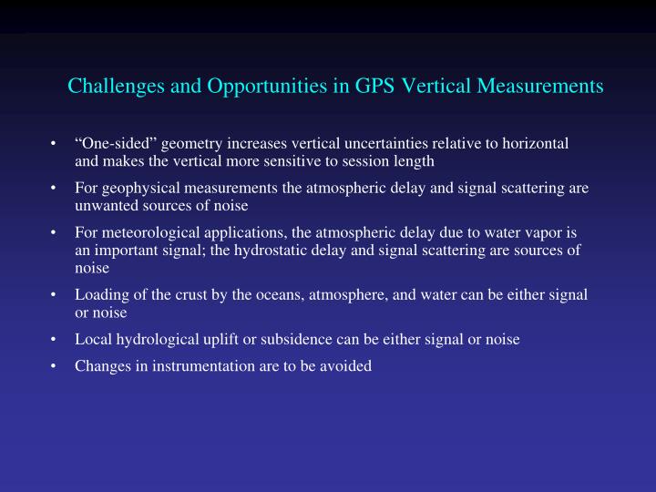
1. Challenges and Opportunities in GPS Vertical Measurements • “One-sided” geometry increases vertical uncertainties relative to horizontal and makes the vertical more sensitive to session length • For geophysical measurements the atmospheric delay and signal scattering are unwanted sources of noise • For meteorological applications, the atmospheric delay due to water vapor is an important signal; the hydrostatic delay and signal scattering are sources of noise • Loading of the crust by the oceans, atmosphere, and water can be either signal or noise • Local hydrological uplift or subsidence can be either signal or noise • Changes in instrumentation are to be avoided

2. Time series for continuous station in (dry) eastern Oregon Vertical wrms 5.5 mm, higher than the best stations. Systematics may be atmospheric or hydrological loading, Local hydrolology, or Instrumental effects

3. Antenna Phase Patterns

4. Modeling Antenna Phase-center Variations (PCVs) • Ground antennas • Relative calibrations by comparison with a ‘standard’ antenna (NGS, used by the IGS prior to November 2006) • Absolute calibrations with mechanical arm (GEO++) or anechoic chamber • May depend on elevation angle only or elevation and azimuth • Current models are radome-dependent • Errors for some antennas can be several cm in height estimates • Satellite antennas (absolute) • Estimated from global observations (T U Munich) • Differences with evolution of SV constellation mimic scale change Recommendation for GAMIT: Use latest IGS absolute ANTEX file (absolute) with AZ/EL for ground antennas and ELEV (nadir angle) for SV antennas (MIT file augmented with NGS values for antennas missing from IGS)

5. Multipath and Water Vapor Can be Seen in the Phase Residuals

6. Top: PBO station near Lind, Washington. Bottom: BARD station CMBB at Columbia College, California

7. Left: Phase residuals versus elevation for Westford pillar, without (top) and with (bottom) microwave absorber. Right: Change in height estimate as a function of minimum elevation angle of observations; solid line is with the unmodified pillar, dashed with microwave absorber added [From Elosequi et al.,1995]

8. Antenna Ht 0.15 m 0.6 m Simple geometry for incidence of a direct and reflected signal 1 m Multipath contributions to observed phase for three different antenna heights [From Elosegui et al, 1995]

9. Sensing Atmospheric Delay the The signal from each GPS satellite is delayed by an amount dependent on the pressure and humidity and its elevation above the horizon. We invert the measurements to estimate the average delay at the zenith (green bar). ( Figure courtesy of COSMIC Program )

10. Zenith Delay from Wet and Dry Components of the Atmosphere Colors are for different satellites Total delay is ~2.5 meters Variability mostly caused by wet component. Wet delay is ~0.2 meters Obtained by subtracting the hydrostatic (dry) delay. Hydrostatic delay is ~2.2 meters; little variability between satellites or over time; well calibrated by surface pressure. Plot courtesy of J. Braun, UCAR

11. Example of GPS Water Vapor Time Series GOES IR satellite image of central US on left with location of GPS station shown as red star. Time series of temperature, dew point, wind speed, and accumulated rain shown in top right. GPS PW is shown in bottom right. Increase in PW of more than 20mm due to convective system shown in satellite image.

12. Water Vapor as a Proxy for Pressure in Storm Prediction Correlation (75%) between GPS-measured precipitable water and drop in surface pressure for stations within 200 km of landfall. GPS stations (blue) and locations of hurricane landfalls J.Braun, UCAR

13. Effect of the Neutral Atmosphere on GPS Measurements Slant delay = (Zenith Hydrostatic Delay) * (“Dry” Mapping Function) + (Zenith Wet Delay) * (Wet Mapping Function) • To recover the water vapor (ZWD) for meteorological studies, you must have a very accurate measure of the hydrostatic delay (ZHD) from a barometer at the site. • For height studies, a less accurate model for the ZHD is acceptable, but still important because the wet and dry mapping functions are different (see next slides) • The mapping functions used can also be important for low elevation angles • For both a priori ZHD and mapping functions, you have a choice in GAMIT of using values computed at 6-hr intervals from numerical weather models (VMF1 grids) or an analytical fit to 20-years of VMF1 values, GPT and GMF (defaults)

14. Percent difference (red) between hydrostatic and wet mapping functions for a high latitude (dav1) and mid-latitude site (nlib). Blue shows percentage of observations at each elevation angle. From Tregoning and Herring [2006].

15. Effect of error in a priori ZHD Difference between a) surface pressure derived from “standard” sea level pressure and the mean surface pressure derived from the GPT model. b) station heights using the two sources of a priori pressure.c) Relation between a priori pressure differences and height differences. Elevation-dependent weighting was used in the GPS analysis with a minimum elevation angle of 7 deg.

16. SShort-period Variations in Surface Pressure not Modeled by GPT Differences in GPS estimates of ZTD at Algonquin, Ny Alessund, Wettzell and Westford computed using static or observed surface pressure to derive the a priori. Height differences will be about twice as large. (Elevation-dependent weighting used).

17. Annual Component of Vertical Loading Atmosphere (purple) 2-5 mm Snow/water (blue) 2-10 mm Nontidal ocean (red) 2-3 mm From Dong et al. J. Geophys. Res., 107, 2075, 2002

18. Atmospheric pressure loading near equator Vertical (a) and north (b) displacements from pressure loading at a site in South Africa. Bottom is power spectrum. Dominant signal is annual. From Petrov and Boy (2004)

19. Atmospheric pressure loading at mid-latitudes Vertical (a) and north (b) displacements from pressure loading at a site in Germany. Bottom is power spectrum. Dominant signal is short-period.

20. Spatial and temporal autocorrelation of atmospheric pressure loading From Petrov and Boy, J. Geophys. Res.,109, B03405, 2004

21. GAMIT Options for Modeling the Troposphere and Loading • For height studies, the most accurate models for a priori ZHD and mapping functions are the VMF1 grids computed from numerical weather models at 6-hr intervals. • For most applications it is sufficient to use the analytical models for a priori ZHD (GPT) and mapping functions (GMF) fit to 20 years of VMF1. • For meteorological studies, you need to use surface pressure measured at the site to compute the wet delay, but this can be applied after the data processing (sh_met_util), and it is sufficient to use GPT in the GAMIT processing • For height studies, atmospheric loading from numerical weather models (ATML grids) should also be applied. (ZHD and ATML are correlated, so don’t use one set of grids without the other)