Download
1 / 43
430 likes | 437 Views
Individual Fitness and Measures of Univariate Selection. In previous lectures, we assumed the nature of selection was known, and our goal was to estimate response. Our interest here is how selection acts on particular phenotypes ( phenotypic selection ). This involves two issues:.

E N D
In previous lectures, we assumed the nature of selection was known, and our goal was to estimate response. Our interest here is how selection acts on particular phenotypes (phenotypic selection) This involves two issues: • Measurement of fitness in individuals • Quantification of any association between fitness and trait values
Episodes of Selection Selection often broken into components, or episodes of selection. Viability selection (differences in survivorship) Fertility selection (differences in number of offspring/mating) Natural vs. sexual selection Sexual selection results from variance in mating success.
Assigning Fitness Components Longitudinal studies, which follow a cohort of individuals through time, are strongly preferred when possible. Cross-sectional studies examine individuals at a single point in time, and typically return only two fitness classes (e.g., dead/alive, mated/unmated). Their analysis requires a considerable number of assumptions. To see how fitness components are assigned when there are several episodes of selection, suppose we measure a cohort of n individuals (indexed by 1 < r < n) over several episodes of selection One must remember that considerable selection may have already occurred prior to our study.
n X 1 W = W ( r ) 1 1 n r =1 The relative fitness is just wj(r) = Wj(r) /Wj Let Wj(r) denote the fitness of individual r for the j-th episode of selection. For example, W could be 0 or 1 (dead/alive), or number of mates, or number of offspring At the start of our study, all individuals are equally- weighted, so that the mean fitness for episode 1 is Thus after the first episode of selection, the r-th individual now has a fitness-weighted frequency of (1/n) w1(r)
) ) ( ( µ ∂ n X 1 W = W ( r ) ¢ w ( r ) ¢ * * 2 2 1 n r =1 µ n X … 1 - - W = W ( r ) ¢ w ( r ) ¢ w ( r ) ¢ ¢ ¢ w ( r ) ¢ j j j ° 1 j ° 2 1 n r =1 Fitness of individual r pj(r), the fitness-weighted frequency of r at the start of the j-th episode j Y 1 - p ( r ) = w ( r ) ¢ p ( r ) = w ( r ) * j j j ° 1 i n i =1 Thus, the mean fitness for episode 2 is the average of the fitness of individuals times their frequencies, In general, the mean fitness for episode j is In particular,
X W = W ( r ) ¢ p ( r ) - * X j j j ° 1 2 2 E [ z ( j )] = z ( r ) ¢ p ( r ) * j X π = z ( r ) ¢ p ( r ) * j z ( j ) - 2 2 2 æ ( z ) = E [ z ( j )] ° π j z ( j ) We can also write the mean fitness of the j-th episode as With the fitness-weighted frequencies for individuals after j episodes of selection, we can compute the fitness-weighted trait means and variances.
µ ∂ ) ( 1 7 W ( r ) 1 W = 1+1+0 +2+3 = = 1 : 4 ; giving w ( r ) = 1 1 5 5 1 : 4 X * W = W ( r ) ¢ p ( r ) 2 2 1 * * * * = (25 ; 820 ¢ 0 : 143) + (22 ; 670 ¢ 0 : 143) + (7 ; 230 ¢ 0 : 286) + (15 ; 986 ¢ 0 : 429) = 15 ; 860 z (1) = 145 ¢ 0 : 143+128 ¢ 0 : 143+ 148 ¢ 0+138 ¢ 0 : 286+141 ¢ 0 : 429 = 138 : 996 * * * * * 2 2 2 2 2 2 z (1) = 145 ¢ 0 : 143+128 ¢ 0 : 143+ 148 ¢ 0+138 ¢ 0 : 286+141 ¢ 0 : 429 = 19 ; 325 * * * * * 5 - 2 V ar [ z (1)] = (19 ; 325 ° 138 : 996 ) = 6 : 39 4 Example: Howard’s (1979) data on mating success (number of mates) W1 and eggs per mating (W2) for male bullfrogs (Rana) as a function of their size
Variance in Individual Fitness How can we compare the amount of selection acting on different populations (independent of the actual traits under selection)? While the selection intensity i allows us to compare different populations, it is character-specific Further, selection can occur without changing the mean (such as stabilizing selection) A character-independent measure for the overall strength of selection on a population that is trait- independent is I, the opportunity for selection,
2 æ 2 W I = æ = w 2 W ≥ ¥ ( ) n - b 2 I = V ar ( w ) = w ° 1 - n ° 1 I is just the variance in relative fitness Which can be estimated by I was introduced by Crow (1958), who called it the index of total selection. The term opportunity for selection was introduced by Arnold and Wade (1984a,b) I bounds the maximum possible selection intensity i for any trait in a population.
j æ j j S j < z ;w p j Ω j = = ∑ 1 ; z ;w æ æ æ I z w z p < j i j ∑ I To see this, we first use the Robertson-Price identity, S = s(z,w), namelythat the selection differential is the covariance between trait value and relative fitness Since the absolute value of a correlation is bounded by 1, Thus, the absolute selection intensity is bounded by the square root of I for any character The most that selection can change any trait in one generation is I1/2 phenotypic standard deviations.
) ( 2 2 2 2 2 2 w = (1 = 5) 1 : 162 + 1 : 020 + 0 + 0 : 652 + 2 : 160 = 1 : 496 b 5 - I = (1 : 496 ° 1 ) = 0 : 62 4 Example: return to our frog data Here, Hence, Thus for this population, the maximum any trait can change over a single generation is 0.621/2~ 0.71 SD Note that the change in male body size (in SD) was just -0.155, less than 1/5 of the maximum absolute possible change
For any set of individuals, this distribution does not change over traits What does change is the association (i.e. regression) of trait value on fitness, s(w,z)/s2z = S/s2z Same set of individuals, hence the same distribution of relative fitness values, but different trait = different regression
In some cases, we do not have data on individual fitness, but rather the fitnesses of phenotypic classes. In such cases we can still place a lower bound on I Example: O’Donald looked at selection on wing eyespot number in the butterfly Maniola by comparing the distribution of eyespot number in wild-caught individuals vs. those reared in the lab
1 * * * * W = [ (1 ¢ 124) + (0 : 699 ¢ 67) + (0 : 675 ¢ 34) + (0 : 548 ¢ 10) ] ' 0 : 838 237 1 * * * 2 2 2 2 * 2 W = (1 ¢ 124) + (0 : 699 ¢ 67) + (0 : 675 ¢ 34) + ( 0 : 548 ¢ 10) ' 0 : 736 237 ) ( ° ¢ 237 - 2 V ar ( W ) = 0 : 736 ° 0 : 838 ' 0 : 034 236 0 : 034 b I = ' 0 : 048 2 0 : 838 £ § Hence, I > 0.048, as Var = Var(between groups) + Var(within groups) I = 0.048 + Var(within groups)
If the variance in fitness is not independent of mean fitness W, then comparisons of I values across populations are compromised. - p (1 ° p ) 1 I = ' if p << 1 2 p p Caveats with using I For example, suppose we look over some short time period and score mating vs. not mating. Mean fitness is simply p, the fraction that have mated. As we look over longer time windows, p should increase. In this case, fitness follows a binominal distribution, with mean p and variance p(1-p), giving I as
In this case, as we change our sampling interval, which increases or decreases p, we also change I A second example where there is a lack of independence between mean fitness and variance in fitness is when individual fitness follows a Poisson distribution, in which case the mean = variance, and I = 1/mean fitness Suppose we have a population of 100 males, but only have 5 females mate, giving mean fitness as 0.05. However, if 50 females mate, mean fitness is now 0.5. Differences between I in these two settings come solely from variation in the number of mating females, not any biological differences between males in mating ability.
Describing Phenotypic Selection One way to describe selection on a trait is to compare the (fitness-weighted) distributions before and after an episode of selection In addition to selection on the trait itself, growth (or other ontogenetic changes), immigration, environment change, selection on phenotypically- correlated traits can all shift this distribution We typically speak of fitness surfaces for traits, which map trait value into fitness W(z) = average fitness of an individual with trait value z
W(z) is called the individual fitness surface. The geometry of the fitness surface describes the Nature of selection: • Directional selection: fitness increases (or decreases with trait value) -- linear relationship between fitness and trait value • Stabilizing selection: The fitness surface has a peak --- convexquadratic relationship btw w and z • Disruptive selection: The fitness surface has a valley --- concavequadratic relationship btw w and z
W(z) may vary with genotypic and environmental backgrounds When the fitness of an individual depends on the distribution of trait values of other individuals (e.g, truncation selection, search imagines, dominance hierarchies), fitness is said to be frequency-dependent. The second type of fitness surface is the mean fitness surface, the average fitness given the distribution of phenotypes. As an analogy, we measure breeding values for individuals, while the summary statistic for the population is the additive variance
Individual fitnesses Distribution of phenotypic values, where q = distribution parameters (such as mean & Variance) Z W ( µ ) = W ( z ) p ( z ; µ ) dz While the mean fitness surface depends on all of the parameters of the distribution, how it changes as we change the population mean is usually what is considered.
Thus, we can write the mean after selection as W ( z ) p ( z ) W ( z ) p ( z ) R p ( z ) = = = w ( z ) p ( z ) s W ( z ) p ( z ) dz W Z Z π = z p ( z ) dz = z w ( z ) p ( z ) dz = E [ z w ( z ) ] To see this, first note that the distribution of the trait after selection is s s Thus, we can express the selection differential as - - S = π ° π = E [ z w ( z ) ] ° E ( z ) E ( w ) = æ [ z ; w ( z ) ] s This follows since E(w) = 1, so that m = m*1 = E(z) * E(w) The Robertson-Price Identity Robertson (1966) and Price (1970, 1972) showed that S = cov(w,z), the covariance between relative fitness w and trait value z. This is a completely general relationship and makes no assumptions.
S æ ( z ; w ) Ø = = 2 2 æ æ z z Directional Selection: Directional Differentials (S) And Gradients (b) Changes in the mean (within a generation) are measured by the directional selection differential S and the selection gradient b, where Note that b is the slope of a regression of relative fitness w on trait value z, w = a + b z = 1 + b(z- mz)
µ ∂ @ ln W 2 R = æ * A @ π @ ln W Ø = @ π Since S = bs2z, we can write the breeders’ equation as R = h2 (bs2z) = (s2A /s2z) (bs2z) giving R = bs2A The real importance of b arises when we consider multiple traits (Lecture 13) When phenotypes are normally-distributed and fitnesses are frequency-independent, then (Lande 1976) Thus, b is the gradient (with respect to m) of the mean fitness surface, hence its name
Summary of measures of the within-generation change in the mean For a single character under selection, we have introduced three measures for change in mean S = m* - m i = S/sz b = S/sz2 While these three measures are just scaled values of each other for a single trait, they behave very differently when we consider their vector extensions for multiple traits The (directional) selection differential, the observed change in the mean The selection intensity, the observed, change in the mean in phenotypic standard deviations. The measure for comparing selection on particular traits The selection gradient, the slope of the regression of relative fitness on trait value
) ( - ° - - 2 2 2 2 æ ° æ = æ w ; ( z ° π ) ° S z z z * Observed within-generation change in the phenotypic variance Directional selection decreases the variance, by an amount S2 Robertson-Price like term for quadratic effects - 2 2 2 C = æ ° æ + S z z * Changes in the Variance: The Quadratic Selection Differential C and Quadratic Selection Gradient (g) Now let’s consider changes in variances. At first though, you might consider the variance analogue to S to simply be the within-generation change in variance, s2z* - s2z The problem is that Lande and Arnold (1983) showed that Based on this expression, Lande & Arnold defined the quadratic selection differential C by
Lande and Arnold originally called C the stabilizing selection differential, but (for a variety of reasons to be discussed) quadratic is much less misleading Note that since directional selection reduces the variance • A reduction in variance is not, by itself, an indication that stabilizing (or more properly convex) selection has occurred. • An increase in variance due to disruptive (or more properly concave) selection can be masked by a decrease in the variance from directional selection (a change in the mean) has occurred.
Example: natural selection in Darwin’s finches on Daphne Major Island (Galapaogos) Boag and Grant (1981) observed intense selection on body size in Geospiza fortis during a severe drought The mean and variance of 642 adults before the drought were 15.79 and 2.37. The mean/variance of the 85 surviving adults was 16.85 / 2.43. Their appeared very little selection in the variance (2.43 - 2.37 = 0.06) However, S = 16.85 - 15.79 = 1.062 , giving the quadratic selection differential as C = 0.06 + 1.062 = 1.14 Hence, a combination of directional and concave (disruptive) selection likely occurred.
Convex / Concave Selection vs. Stabilizing / Disruptive selection Convex selection: The individual fitness surface has a negative curvature Stabilizing selection: The individual fitness surface has a negative curvature AND has a maximum within the range of phenotypes seen in the population Concave selection: The individual fitness surface has a positive curvature. Disruptive selection: The individual fitness surface has a positive curvature AND has a minimum within the range of phenotypes seen in the population
q < - 4 j C j ∑ I ( π ° æ ) 4 ;z z 4-th moment about the mean, E[(x-m)4], -- kurtosis p < 2 j C j ∑ æ 2 I z Since C = s[ w, (z- mz)2 ], we can also use arguments akin to leading to a bound on S based on I, the opportunity for selection Specifically, For a normally-distributed trait, the 4th moment is 3 sz4, giving
£ § ) - ( 2 æ w ; ( z ° π ) C ∞ = = 4 4 æ æ z z Quadratic Selection Gradient (g) The Quadratic Selection Gradient (g) is defined by As we will see shortly, g (like b) is also a coefficient in a fitness regression, here on quadratic terms. Likewise (again like b) g is a measure of the average geometry of the individual fitness surface, in particular The average slope.
Z @ w ( z ) Slope of the individual fitness surface at trait value z Ø = p ( z ) dz @ z Z 2 Curvature of the individual fitness surface at trait value z @ w ( z ) ∞ = p ( z ) dz 2 @ z b and g describe the average geometry of the fitness surface Provided phenotypes are normally distributed, b = average slope, no matter how messy the fitness surface g = average curvature, no matter how messy the fitness surface
2 D π = æ Ø A 4 4 ° ¢ h æ ) ( - 2 2 A D æ = ± = C ° S 2 æ z 4 2 2 æ z z 4 ) æ ( - 2 A = ∞ ° Ø 2 ) ( 4 d ( t ) æ ( t ) - 2 A d ( t +1) = + ∞ ( t ) ° Ø ( t ) 2 2 b and g fully describe the effects of phenotypic selection in the response equations Change in mean Change in variance (one generation of selection) Change in variance (general) ¢
2 Co v ( z ; w ) V ar ( z ) 2 2 b r = = Ø z ;w V ar ( z ) ¢ V ar ( w ) b * I Linear and Quadratic Approximations of W(z) To simplify expressions somewhat we first rescale our trait to have mean zero (i.e, subtract off the mean) The best linear regression predicting relative fitness w given trait value z is w = 1 + bz + e The slope of the best-fitting linear regression is given by s(w,z)/ s2z = b.
Ø Ø 2 Ø Ø @ w ( z ) @ w ( z ) Ø Ø = b ; = 2 b 1 2 2 @ z @ z z = π z = π z z Slope of the fitness surface evaluated at the mean is b1 (1/2)b2 is the curvature of the surface at the mean Now consider the best quadratic regression w = 1 + b1z + b2z2+ e The regression coefficients b1 and b2 nicely summarize the local geometry Ø Ø What are b1 and b2 for the best-fitting regression? b1 is NOT necessarily b!
An interesting feature of quadratic selection is that it can result in a change in the mean, even when no direct selection on the mean is apparent. Both populations are under strict stabilizing selection, with the mean under the optimal value q. The phenotypic distribution on the left is symmetric and does not experience directional selection. However, the population on the right has skew it its phenotypic variance, and hence the stabilizing selection unevenly shifts the distribution after selection, resulting in a change in mean
- - - 2 4 * * æ ( x ) ¢ æ ( x ; w ) ° æ ( x ; x ) ¢ æ ( x ; w ) ( π ° æ ) ¢ S ° π ¢ C * * 2 1 1 2 2 4 ;z 3 ;z z b = = - - - 1 2 2 2 2 2 4 æ ( x ) ¢ æ ( x ) ° æ ( x ; x ) æ ¢ ( π ° æ ) ° π * 1 2 1 2 4 ;z z z 3 ;z - - 2 2 * * * æ ( x ) ¢ æ ( x ; w ) ° æ ( x ; x ) * ¢ æ ( x ; w ) æ ¢ C ° π ¢ S 1 2 1 2 2 3 ;z z - - b = = If skew is present, the linear slope is influenced by the quadratic selection differential. Likewise the quadratic slope is influenced by the directional selection differential. - 2 2 2 2 2 2 4 * * æ ( x ) ¢ æ ( x ) ° æ ( x ; x ) æ ¢ ( π ° æ ) ° π 1 2 1 2 4 ;z z z 3 ;z Find the regression coefficients by OLS Using the results from Lecture 2 for y = a + b1x1 + b2x2 gives If skew is absent, b2 = C/(m4z - sz4). If z is normally distributed, then m4z - sz4 = 3sz4 - sz4 = 2sz4, giving b2 = C/(2sz4) = g/2 If skew is absent, b1 = b. Thus, when z is normal, the regression reduces to w = 1 + bz + (g/2)z2+ e This is the Lande-Arnold regression, or Lande-Arnold fitness estimation.
Nonparametric estimators of the fitness surface If the fitness surface have higher order curvature beyond the quadratic, the fitted quadratic regression terms can be potentially misleading. For example, with multiple peaks/values, a quadratic regression assumes (at most) only one extreme point. This has lead to nonparametric (distribution-free) estimates of the fitness (response) surface. Schulter (1988) produced a method using a local series of splines (cubic polymonials) Thin-plate spline methods have also been used, fitting “plates” instead of lines
Complications with Unmeasured Variables As we will discuss in Lecture 14, our estimates are biased if there are traits under selection that are phenotypically correlated with our trait. Happily, traits under selection that are not phenotypically correlated do not bias our results (even if they are genetically correlated) An interesting example is Kruuk etal. (2002) who looked at antler size in red deer. For example, suppose plants in good soil environments produce both larger plants and more seeds. If we do not know soil type, we will assume larger plants have a higher fitness. A potentially more serious issue is when the environment influences both our trait and also fitness. Males with larger antlers enjoy increased lifetime breeding success (antlers being involved in male- male competition), resulting in a b = 0.44 + 0.18 Further, antler size is also heritable, h2 = 0.22 + 0.12 Despite selection and heritability, no observed response over 30 years of study Authors suggest that antler size and male fighting ability heavily dependent upon an individual’s nutritional state
How Strong is Selection in Natural Populations? Bumpus (1899) and Weldon (1901) were the first to publish attempts to detect selection on quantitative traits in nature Endler (1986) was the first to make a serious attempt at summarizing the average strength of selection Kingsolver and colleagues (2001) provide the most recent summary, with other 2,500 estimates of b and g from natural populations
b values fit an exponential distribution, with medium (50%) values of scaled b = 0.16. This means that a one SD change in the trait changes fitness by 16% Selection is generally weak, with few (<10%) of the b > 0.5 Most large estimates of b occur in small populations. For samples sizes > 1000, most estimates of b are below 0.1
Medium value of |g | was 0.10 Distribution of the estimated g is symmetric, with concave (“disruptive”) selection (g < 0) as common as convex (“stabilizing”) selection (g > 0). Blows & Brooks (2003) point out issues with estimating selection from the gii terms in a multivariate analysis (we will return to this)
The Importance of Experimental Manipulation As we have tried to stress, unmeasured (but phenotyically correlated) traits, environmental factors that influence both the trait and fitness, changes in the environment and additional complications (such as inbreeding depression) can seriously bias estimates of fitness-trait associations. Hence, the final analysis should always try to include direct experimental manipulation to demonstrate that a detected correlation really has a direct effect.