Download
1 / 51
510 likes | 709 Views
The ALFA project in ATLAS. Antwerpen 25/10/07 Per Grafstrom. ATLAS FORWARD DETECTORS. Purpose of ALFA. Additional handle on the luminosity ALFA = Absolute Luminosity For ATLAS Measurement of tot and elastic scattering parameters Tag proton for single diffraction.

E N D
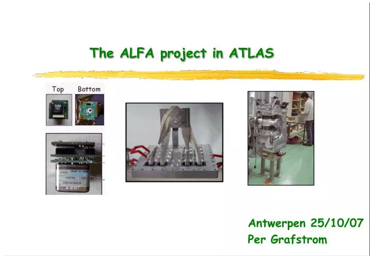
The ALFA project in ATLAS Antwerpen 25/10/07 Per Grafstrom
Purpose of ALFA • Additional handle on the luminosity • ALFA = Absolute Luminosity For ATLAS • Measurement of tot and elastic scattering parameters • Tag proton for single diffraction
Luminosity measurements-why? • Cross sections for “Standard “ processes • t-tbar production • W/Z production • ……. Theoretically known to better than 10% ……will improve in the future • New physics manifesting in deviation of x BR relative the Standard Model predictions • Important precision measurements • Higgs production x BR • tan measurement for MSSM Higgs • …….
Relative precision on the measurement of HBR for various channels, as function of mH, at Ldt = 300 fb–1. The dominant uncertainty is from Luminosity: 10% (open symbols), 5% (solid symbols). (ATLAS-TDR-15, May 1999) Examples Higgs coupling tan measurement Systematic error dominated by luminosity (ATLAS Physics TDR )
Elastic scattering as a handle on luminosity • optical theorem: forward elastic rate + total inelastic rate: • needs large |η| coverage to get a good measurement of the inelastic rate- otherwise rely on MC in unmeasured regions • Use totmeasured by others (TOTEM) • Combine machine luminosity with optical theorem • luminosity from Coulomb Scattering ATLAS pursuing all options
Absolute vs relative measurement • STRATEGY: 1. Measure the luminosity with most precise method at optimal conditions 2. Calibrate luminosity monitor with this measurement, which can then be used at different conditions • Relative Methods: • LUCID (dedicated luminosity monitor) • BCM • Min. Bias Scintillators • Tile/LAr Calorimeters
Elastic scattering at small angles • Measure elastic rate dN/dt down to the Coulomb interference region (à la UA4). |t|~0.00065 GeV2 or Θ ~ 3.5 microrad. This requires (apart from special beam optics) • to place detectors ~1.5 mm from LHC beam axis • to operate detectors in the secondary vacuum of a Roman Pot • spatial resolution sx = sy well below 100 micron (goal 30 micron) • no significant inactive edge (< 100 micron)
Elastic scattering All very simplified – we need Electromagnetic form factor Proper treatment of the Coloumb-hadron interference phase t- dependence of rho and phase non-exponential behaviour -t dependence of the slope Saturation effects
=2.2 (best fit) ) totvs sand fit to (lns) =1.0 The total cross section Alan Valery Mishka
The ρ parameter • ρ = Re F(0)/Im F(0) linked to the total cross section via dispersion relations • ρ is sensitive to the total cross section beyond the energy at which ρ is measured predictions of tot beyond LHC energies is possible • Inversely :Are dispersion relations still valid at LHC energies? (Figures from Compete collaboration)
The b-parameter for lt l< .1 GeV2 “Old” language : shrinkage of the forward peak b(s) 2 ’ log s ; ’ the slope of the Pomeron trajectory ; ’ 0.25 GeV2 Not simple exponential dependence of local slope Structure of small oscillations? The b-parameter or the forward peak
Single Diffraction elastic scattering RP RP RP RP 240m 240m IP RP RP RP RP single diffraction ATLAS RP RP LUCID LUCID RP RP ZDC ZDC IP RP RP LUCID ATLAS LUCID RP RP ZDC ZDC 240m 140m 17m 17m 140m 240m
Trigger conditions • For the special run (~100 hrs, L=1027cm-2s-1) • 1. ALFA trigger • coincidence signal left-right arm (elastic trigger) • each arm must have a coincidence between 2 stations • rate about 30 Hz • 2. LUCID trigger • coincidence left-right arm (luminosity monitoring) • single arm signal: one track in one tube • 3. ZDC trigger • single arm signal: energy deposit > 1 TeV (neutrons) • 4. Single diffraction trigger • ALFA.AND.(LUCID.OR.ZDC) • central ATLAS detector not considered for now (MBTS good candidate)
Event generation and simulation PYTHIA6.4 modified elastic with coulomb- and ρ-term single diffraction PHOJET1.1 elastic & single diffraction beam properties at IP1 size of the beam spot σx,y beam divergence σ’x,y momentum dispersion single diffraction L1 filter LUCID & ZDC pre-selection elastic scattering ALFA simulation track reconstruction t-spectrum ξ-spectrum luminosity determination beam transport MadX tracking IP1RP high β* optics V6.5 including apertures (Work of Hasko Stenzel-Giessen)
Hit pattern in ALFA hit pattern for 10 M SD events simulated with PYTHIA + MADX for the beam transport Dispersion
acceptance for t and ξ • global acceptance: • PYTHIA 45 % • PHOJET 40.1 %
MAPMT + VD + RO cards Kapton flat cable motherboard Feedthrough for trigger photodetectors
ALFA 2007: a full scale detection module 23 MAPMTs 10x2 for fiber detector 3x1 for overlap detector Frame from the 2006 TB Base plate similar to the 2006 version, but with central fixation for fiber plates and 1 free slot for triggers feed-through New design for the fiber plates support 3 overlaps fiber plates: New substrates design 10-2-64 fiber plates: New substrates design Trigger scintillators:
The test beam at DESY • the validity of the chosen detector concept with MAPMT readout • the baseline fibre Kuraray SCSF-78 0.5 mm2 square • expected photoelectric yield ~4 • low optical cross-talk • good spatial resolution • high track reconstruction efficiency • No or small inactive edge • Technology appears fully appropriate for the proposed measurement. Conclusions from DESY test beam
Time line • Mechanics • Prototype tested • Full production launched • Delivery end February 2008 • Detector • A number of small prototypes tested • Construction of one full detector started (1/8 of total system) • Production start after validation spring 2008. • Full detector in 2009 • Electronics • Prototypes tested • Electronics corresponding to one full detector by end 2007 • All electronics by end 2008
Simulation of the LHC set-up elastic generator PYTHIA6.4 with coulomb- and ρ-term SD+DD non-elastic background, no DPE beam properties at IP1 size of the beam spot σx,y beam divergence σ’x,y momentum dispersion ALFA simulation track reconstruction t-spectrum luminosity determination later: GEANT4 simulation beam transport MadX tracking IP1RP high β* optics V6.5 including apertures
Acceptance distance of closest approach to the beam Global acceptance = 67% at yd=1.5 mm, including losses in the LHC aperture. Require tracks 2(R)+2(L) RP’s. Detectors have to be operated as close as possible to the beam in order to reach the coulomb region! -t=6·10-4 GeV2
L from a fit to the t-spectrum Simulating 10 M events, running 100 hrs fit range 0.00055-0.055 large stat.correlation between L and other parameters
Simulation of elastic scattering hit pattern for 10 M elastic events simulated with PYTHIA + MADX for the beam transport t reconstruction: • special optics • parallel-to-point focusing • high β*
t- and ξ-resolution: PYTHIA vs PHOJET • Good agreement between PYTHIA and PHOJET for the reolutions
reconstruction bias • True and reconstructed values are in average slightly shifted • needs to be corrected • some differences observed at small t
Introduction – physics case • single diffraction ppX+p: • complements the elastic scattering program • measurement of cross section and differential distributions • fundamental measurement, tuning of models, background determination • special detectors ALFA+LUCID+ZDC • high β* optics • same special run as for luminosity calibration
resolution for t and ξ • main contribution to the resolution • t: vertex smearing, beam divergence (small t), det. resolution (large t) • ξ: vertex smearing and detector resolution
Systematic uncertainties • generator difference, model dependence • acceptance, detector corrections ± 5-10% • beam conditions, optical functions, alignment • ± 2% (based on results for elastic scattering) • background (being estimated) • double diffraction • minimum bias • beam halo • DD ≈ 2 %, MB ≈ 0.5 %, beam halo + DD/MB 1-2% • luminosity • ± 3%, very best possible luminosity determination, at calibration point! • statistical uncertainty small, expect 1.6-2.3 M accepted events
Conclusion & outlook • A measurement of single diffraction with ATLAS appears to be possible, • however it won’t be a precision measurement in contrast to elastic • scattering. • Combination ALFA, LUCID and ZDC • Special running conditions • measurement of cross section and t-, ξ-distribution • not a precision measurement, 10% systematic uncertainty achievable? • goal: improve model predictions and background estimates for central diffraction • This first pilot study must be pursued and confirmed by full simulation and • systematic studies involving the LUCID and ZDC communities. The option of • including the MBTS for tagging the diffractive system should be investigated.
Systematic errors • Background subtraction ~ 1 % Background subtraction ~ 1%
Luminosity transfer 1027-1034 cm-2 sec-1 • Bunch to bunch resolution we can consider luminosity / bunch ~ 2 x10⁻⁴ interactions per bunch to 20 interactions/bunch • Required dynamic range of the detector ~ 20 • Required background < 2 x10⁻⁴ interactions per bunch • main background from beam-gas interactions • Dynamic vacuum difficult to estimate but at low luminosity we will be close to the static vacuum. • Assume static vacuum beam gas ~ 10-7 interactions /bunch/m • We are in the process to perform MC calculation to see how much of this will affect LUCID
t-resolution The t-resolution is dominated by the divergence of the incoming beams. σ’=0.23 µrad ideal case real world