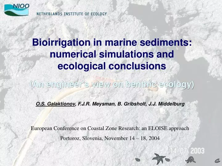
Bioirrigation in marine sediments: numerical simulations and ecological conclusions

1. Bioirrigation in marine sediments:numerical simulations andecological conclusions (An engineer's view on benthic ecology) O.S. Galaktionov, F.J.R. Meysman, B. Gribsholt, J.J. Middelburg European Conference on Coastal Zone Research: an ELOISE approach Portoroz, Slovenia, November 14 – 18, 2004

2. Modelling (bio)-irrigation in permeable aquatic sediments • Types of sediments: • muddy (low permeability): solute transport is dominated by diffusion • sandy (high permeability): advective transport by porewater flows may far exceed the magnitude of diffusive fluxes water column sediment • (Bio)-irrigation: • passive • advection caused by the interaction of the overlying water flow with (biogenic) bedforms, i.e. ripples, mounds, protruding shells etc. • diffusion through the burrow walls etc. • active advection of porewater due to activity of benthic organisms†: ventilation of burrows etc. † Activity of benthic organisms may also enhance diffusive transport (through the tube walls)

3. Active bio-irrigation (by the lugworm Arenicola marina) Schematic drawing of Arenicola in its burrow Importance of the quicksand channel (higher permeability) should be examined

4. How complex the bio-irrigation model geometry should be? 3D 2D axisymmetric 1D • retainsfull spatial complexity • computationally expensive • necessarily low resolution • faster FEM simulations • allows high resolution • retains sufficient complexity • very fast simulations • no downward advection • no horizontal heterogeneity

5. Bio-irrigation by the Arenicola marina: importance of burrow insulation Permeable burrow walls: flow shortcuts, anoxic pore water re-enters the burrow Insulated burrow walls: only overlying water is drawn to the burrow Burrow wall insulation helps to extend habitat towards less permeable sediments • Active insulation: lining burrow walls with mucus, “head banging” etc.requires investment of resources • Passive insulation: accumulation of iron oxides etc.is “free” but costs time – may explain the semi-permanent nature of the burrows

6. 3D, 2D and 1D models: meshes and streamlines 3D 2D axisymmetric 1D* actual mesh and streamlines actual mesh and streamlines * sketch

7. Numerical models of bio-irrigation are applied to: Injection experiment Flushing experiment Field study Measuring tracer appearance in overlying water Tracer addition (Br- ) sea organic matter Br- NO3-? O2 SO42- rough sand NO3-, O2 aquifer NO3- Saturation of pore water with tracer (NO3-) Measure tracer appearance in pore water Saturating pore water with tracer (NO3- )

8. Modelling Br- injection: coupled 2D axisymmetric model (unamended) Horizontally averaged tracer profiles Computed concentration patterns • Overlying water column is assumed to be ideally mixed • t = 96 min is actual incubation time; no tuning of the parameter values!

9. Reproducing the core incubation data with 3D, 2D and 1D models Small feeding pocket Amended models (vertically enlarged feeding pocket) • 2D model can be easily tuned by adjusting the feeding pocket geometry • 1D model also requires strong additional non-mechanistic tuning: increasing the effective diffusivity (hydromechanical dispersion)

10. Approximating Timmermann (2002) results: large feeding pocket (?)

11. Experimental artifacts(?): flushing nitrate from the sediment core • NO3- flushing test: • sediment core saturated with nitrate solution; • overlying water replaced (by clean water); • one Arenicola marina introduced; • nitrate concentration in water column monitored • Conclusions: • Concentration overshot (core 1) is reproduced by the model • Presence of the overshot is controlled by the core geometry • Flow is essentially 3D: layers below the burrow are efficiently flushed

12. Bio-irrigation and NO3- transport to the sea (NAME project) Field site (Denmark): … sea organic matter NO3-? O2 SO42- rough sand NO3-, O2 aquifer What is the role of bio-irrigation?

13. Bio-irrigation and NO3- transport to the sea (NAME project) └─ organic matter ─┘ oxygen sulfate nitrate H2S The computed concentration patterns correspond to the discharge velocity 2 m/yr and worm density 8 m-2 (each pumping 1ml/min) Preliminary remarks • Nitrate is prevented from the contact with the large part of organic matter • Zone clear from nitrate is irrigated with abundant sulfate (sea water) • Hydrogen sulfide production may result from bio-irrigation

14. NO3- transport to the sea: influence of discharge velocity from aquifer • Advective bio-irrigation strongly affects the nitrate removal / discharge into the sea • NO3- consumption is suppressed by mechanical separation of nitrate-rich aquifer water from reactive organic matter • Reliable prediction of nitrate removal requires simultaneous knowledge of the aquifer discharge rate and animal density/activity

15. Bioirrigation in marine sediments: Concluding remarks • Sediment permeability is the key factor shaping the ecology of the marine sediments • Arenicola marina • Burrow lining prevents flow short-circuits, extends habitat to less permeable sediments • Advective bio-irrigation reaches the sediment layers below the burrow depth • Advective bio-irrigation: 3D → 2D → 1D(?) model • 3D model is computationally expensive, prohibiting high resolution • 2D axisymmetric model: • captures important features of the flow, including advective flow below the burrow • computationally efficient, still allowing high resolution • 1D modelrequires excessive tuning: uses enhanced diffusion to mimic advective effects Application: advective bio-irrigation and NO3- removal • Animal activity (bio-irrigation) may hinder the nitrate removal • Reliable predictions require data on both aquifer discharge rate and animal density/activity Thank you for attention!

16. Additional sides

17. Bio-irrigation by the Arenicola marina: importance of burrow insulation Insulatedburrow walls only overlying water is drawn to the burrow Permeable burrow walls: flow shortcuts, anoxic pore water re-enters the burrow Streamlines of the porewater flow, computed in the assumption of uniform sediment properties. Numerical simulations show the importance of the burrow lining: it allows to extend habitat to less permeable sediments

18. Bio-irrigation (by the lugworm Arenicola marina): quicksand importance? Computed depth profile for the concentration of passive tracer (laterally integrated from 3D-simulations) compared to the experimental data obtained by Timmermann et al., (2002) Comparing the computed passive tracer profiles in the cylindrical core with and without quicksand column (10 times higher permeability)

19. Bio-irrigation by the Arenicola marina: importance of burrow geometry By placing a finite size source at the axis of axisymmetric sediment core the dependence of the sediment resistance of the burrow geometry was evaluated • Facts, revealed by simulations: • resistance slowly grows with the burrow depth (most of it happens near the source) • burrow opening (size of feeding pocket) plays a larger role • We may speculate that: burrow depth is likely determined by other factors (food availability, predator avoidance…), while it is advantageous for a worm to enlarge the feeding pocket to facilitate pumping.

20. Diffusive versus advective bio-irrigation Classical description of bio-irrigation: tube model (Aller, 1980) passive irrigation (diffusion) Alternative (complementary?) description of bio-irrigation: active irrigation (advection) ◄ combination of these models? ►

21. Simple model of advective bioirrigation: source in the cylindrical domain The velocity field (described by Darcy’s law) in the cylindrical domain with open upper side that contains a point source at the axismay be obtained analytically: Comparison (pressure contours) of the analytical and FEM solutions (FEMLAB): Where and βk are the roots of the Bessel function: J and I are Bessel functions and modified Bessel function of the 1st kind Coefficients an, b0 and bkare defined so that the boundary conditions are fulfilled on the walls

22. Bio-irrigation and reactive tracers: 3D effects versus 1D approximations • From 3D to 1D: • flow patterns in axisymmetric core with a small source • steady state distribution of decaying tracer • averaging concentration field horizontally to obtain 1D profile • Next step: • Can the resulting concentration profile vs. depth be reproduced in the 1D reactive transport model?

23. Linearly decaying tracer: Gaussian distributed source in 1D Horizontal averaging preserves the linear relation between concentration and reaction rate: Tracer concentration profile averaged from axisymmetric simulations is well matched by 1D Gaussian distributed source

24. 1D vs. 3D (linearly decaying tracer): effective width of 1D source The problem of the best-fit source width includes five parameters: source widthσ [L], source depthX0 [L], core radiusRc[L], reaction rate constantk [T-1]and source intensityF* [L3T-1]with two independent dimensionalities (length L and time T). According to Buckingham’s Π theorem non-dimensional source width σ′ = σ / X0 should depend on only two independent non-dimensional parameters: Note: the approx. formula represents merely a good fit and was notanalytically derived

25. 1D vs. 3D, (nearly) zero-order reaction: more questions than answers… Zero-order reaction rate is approximated by the monod-type expression Reference case: • Horizontal averaging (3D → 1D) leads to a gross overestimation of the total reaction rate • Secondary effect: shift of the concentration maximum towards sediment-water interface • Adjustment of the reaction rate constant is required for the 1D model • The best fit is achieved with a more “linearized” dependence of R(c)

26. Bio-irrigation (by the lugworm Arenicola marina): quicksand importance? Better fitting (Timmerrmann, 2002; core 2e) using quicksand: • Diameter of the column with higher permeability and the change in permeability are merely fitting parameters (not properly observed or measured) • Not all cases are properly described using only this assumption

27. Flushing tracer from the sediment core: numerical predictions Screen snapshot:

28. Passive (bio)-irrigation: porewater flow under the seabed form (ripple) Pressure variations, arising around the obstacle in the near-bottom flow drive the porewater fluxes under the obstacle Experimental images from Huettel M. et al , Limn. And Ocean. 41 (2), 1996: The images above were taken at the intermediate range of Re (near transition to turbulence) The porewater flow under the ripple at different flow regimes can be simulated numerically…

29. Passive irrigation: porewater flow under the seabed form (ripple) Pressure variations, arising around the obstacle in the near-bottom flow drive the porewater fluxes under the obstacle Laminar flow (Re ≈ 200) v ~ 1 cm/s: Porewater velocity at z=0 under the ripple crest is aprox. 0.036 mm/h log U Turbulent flow (Re ≈ 5000) v ~ 25 cm/s : Porewater velocity at z=0 under the ripple crest is aprox. 5 cm/h

30. Simple model of advective bioirrigation: source in the cylindrical domain has the solution in the form where with the coefficients:

31. Bio-irrigation and NO3- transport to the sea (NAME project) Chem. species:O2, Fe2+, SO42-, HS-, CH4, HCO3-, NO3-, N2, Cl-, DOM ; CH2O, FeOOH, FeS Reactions set: mineralization Conservation equations have a form: Di – diffusion/bioturbation coefficient, ui – advection/burial velocity, Ri – reaction rate