Download
1 / 46
460 likes | 464 Views
Gaia ITNG2013 School, Tenerife Ken Freeman, Lecture 5: the Galactic Bulge chemical tagging and GALAH. The Galactic Bulge Morphology Metallicity distribution Kinematics. The ARGOS survey: goal is to see if the boxy Galactic bulge

E N D
Gaia ITNG2013 School, Tenerife Ken Freeman, Lecture 5: the Galactic Bulge chemical tagging and GALAH The Galactic Bulge Morphology Metallicity distribution Kinematics The ARGOS survey: goal is to see if the boxy Galactic bulge is consistent with the expectations for a bulge that grew from the disk via bar-buckling instabilities.
Melissa Ness The ARGOS bulge survey Freeman, Ness, Bland-Hawthorn, Athanassoula, Asplund, Wylie, Lewis, Yong, Ibata, Kiss, Lane A spectroscopic survey of 28,000 giants in the bulge and the adjacent disk, to measure the kinematics and chemical properties of stars (Fe, Mg, Si, Ti, Al, O) in the bulge and adjacent disk. AAOmega fiber spectrometer on the AAT: CaT spectra of about 350 stars at a time : R ~ 11,000, S/N > 70 per resolution element.
In the bar-buckling instability scenario, the bulge structure is younger than its oldest stars, which were originally part of the inner disk. In the N-body simulations, it takes about 2 Gyr for the bar to form in the disk and then to buckle. So, the stars of the bar/bulge may be chemically similar to stars of the adjacent thin and thick disk that are about 8 Gyr old.
The 28 fields cover the southern bulge (b = -5, -7.5, -10o) plus 3 relatively transparent northern bulge fields, and extend out into the adjacent disk and thick disk 28 fields 1000 stars per field
l = +20 l = -20 Bulge survey lines of sight pass through several structures. Expect to see thin disk,thick disk, bulge, halo, spiral arm populations
Goals of the observational program • measure accurate radial velocities, metallicities and -abundances for stars throughout the southern bulge and adjacent disk. Then compare with dynamical and chemical models of different kinds of bulges. • the stars are selected to • cover the whole line of sight through the bulge at each (l,b) •investigate bulge dynamics, and kinematical and chemical relationship between bulge and disk. • include candidate metal-poor giants to evaluate the contribution of the metal-poor halo and potential first stars in the bulge region. •provide enough stars to detect a 5% classical (spheroidally-rotating) component from its kinematics
To study the bar/bulge, we want to reduce contamination by foreground and background stars, so photometric or spectroscopic distances are important. Ideally use stars for which reasonably accurate distances can be derived. Bright giants are not ideal. Clump giants are good: they have narrow range of absolute magnitude around MK = -1.61 with = 0.22 about the mean. From ARGOS sample, select stars within RG = 3.5 kpc as bulge stars, using isochrone distances from our temperatures and spectroscopic gravities and abundances.
K J-K The sample • mainly red clump stars selected from 2MASS (K, J-K) but also includes brighter giants • color cut is reddening dependent and includes metal-poor giants in the sample • magnitude range covers whole line of sight through the bulge at each (l,b) : about 1000 stars per field in 28 fields. Uniform selection per unit I-magnitude (observing at the Ca triplet). * *
Ca triplet spectra: the I-magnitudes of the stars are between I = 13 and I = 16, selected uniformly in magnitude because 2MASS becomes incomplete for the fainter stars. For each star, we adopt the Schlegel reddening and derive Te, log g, [Fe/H] and [/Fe]. For our fields at |b| = 5 to 10°, E(J-K) ranges from 0.06 to 0.39 (mostly around 0.2) and the Schlegel (1998) and Gonzalez et al (2011) reddening agree well enough. Most of our stars are more than 300 pc from the plane, so expect Schlegel scale to be realistic.
From the spectra, we measure stellar parameters Parameter errors are estimated from observations of independently measured stars in the field, open clusters, globular clusters and bulge: Radial velocity ± 0.9 km s -1 Te ± 100K [Fe/H] ± 0.09 [/Fe] ± 0.10 log g ± 0.30 Of our 28,000 stars, about 2500 are foreground dwarfs and 11,500 are giants outside the inner 3.5 kpc which we take as our bulge region. Only half of the sample are giants in the bulge region.
sun bulge Which stars contribute to the boxy peanut structure of the bulge ? See two peaks in the distribution of bulge stars along the line of sight, but only for stars more metal-rich than [Fe/H] = -0.5. Stars with [Fe/H] < -0.5 are not part of this peanut structure.
The MDF generalised histograms show 5 components for RG < 3.5 kpc 4200 2000 4000 [Fe/H] A 0.12 ± 0.02 B -0.27 ± 0.02 C -0.70 ± 0.01 D -1.18 ±0.01 E -1.68 ± 0.05 A is strong, C is weak at l = -5 A is weak, C is strong at l = -10
Same MDFs as conventional histograms, with same gaussian components. RG < 3.5 kpc. See change of relative weights with latitude Bayesian Information Criterion gives optimal number of components between 4 and 5 These same components are seen all over the bulge and surrounding disk
MDFs on the minor axis: l = 0 See the metallicity gradient as seen by Zoccali et al (2008). See weak tail of metal-poor stars usually excluded by selectic criteria The individual components A,B,C have small negative metallicity gradients in R and z. The apparent abundance gradient in z comes from the changing contributions of components A-C with z-height above the plane.
The MDF in the disk field at l = -31º, b = -5º (RG = 4.0 to 4.9 kpc) All components are present in this field outside the bulge: weights are similar to those for the b = -5º bulge fields. In this inner disk field, these three components are probably present in their undisturbed form, as disk stars, while in the bulge fields the stars of these components have been trapped dynamically into the bulge.
Alpha element abundances (RG < 3.5 kpc) -5º -10º Component A is weakly -enhanced and is strongly involved in the peanut bar/bulge structure. It could be the colder more metal-rich part of the early thin disk. B is -enhanced and is the main component of the bar/bulge. C is -enhanced and not involved in the peanut bar/bulge structure. It may the early inner thick disk.
l = -31º, b = -5º Interpretation of components The disk took ~ 2 Gyr to evolve chemically and dynamically before going unstable and buckling into the peanut structure, so the components A-E are trapped relics of the Galactic disk and halo from that time. The instability process generated a mapping of the stars of the early disk into the boxy/peanut structure. In this way, the bulge preserves a dynamical imprint of the chemical distribution of the disk at the time that the buckling occurred. The bulge is a chemical snapshot of the MDF of the early disk captured in the bar. The mapping of disk into bulge depends on the location and motions of the stars at the time of the instability. Kinematically colder stars can suffer strong radial and vertical migration, and can therefore be strongly involved in the peanut structure (components A and B). (Some of these bulge MDF components were seen in smaller samples of bulge stars by Babusiaux et al 2010)
Kinematics of the bulge components VGC is stellar l.o.s. velocity corrected for the sun’s peculiar motion and the motion of the LSR ARGOS and BRAVA data show the near-cylindrical rotation, as expected for a boxy bulge.
VGC A B C Kinematics of components A-C ([Fe/H] > -1) • B rotates a bit more rapidly than A and is hotter • A and B have similar shape of (l,b) but A < B. (C different) • A is probably more radially concentrated than B
VGC Kinematics of components D and E ([Fe/H] < -1) Rotation of the metal poor stars is much slower and the dispersion is higher : Dynamical different populations from components A-C
HERMES isa new high-resolution fiber-fed multi-object spectrometer on the AAT spectral resolution 28,000 (also R = 45,000 mode) 400 fibres over square degrees 4 bands (BGRI) ~ 1000 Å First light late 2013 Main driver: the GALAH survey (Galactic Archaeology with HERMES)
Using chemical tagging, try to find the debris of groups of stars, now dispersed, that were associated at birth, either • because they were born together in a single Galactic star-forming event, or • because they came from a common accreted galaxy. A major goal is to identify how important mergers and accretion events were in building up the Galactic disk and the bulge.
The galactic disk shows kinematical substructure : usually called moving stellar groups. The stars of the moving groups are all around us • Some are associated with dynamical resonances (eg Hercules moving group) • Some are debris of star-forming aggregates in the disk (eg the chemically homogeneous HR1614 and Wolf 630 moving groups), dispersed into extended regions of the Galaxy • Others may be debris of infalling objects, as seen in CDM simulations
V U Hercules HR1614 De Silva et al 2007
Hercules group o Field stars • The chemical abundances of Hercules Group stars cannot be distinguished from the field stars. This is a dynamical group, not the relic of a star forming event. Bensby et al 2007
• HR 1614 o field stars The HR 1614 stars (age 2 Gyr) are chemically homogeneous. They are probably the dispersed relic of an old star forming event. De Silva et al 2007
Although the disk does show some surviving kinematic substructure in the form of moving stellar groups, a lot of dynamical information was lost in the the subsequent heating and radial mixing by spiral arms and giant molecular clouds. Most dispersed aggregates would not now be recognizable dynamically However ... we are not restricted to dynamical techniques. Much fossil information is locked up in the detailed distribution of chemical elements in stars.
Chemical Tagging Use the detailed chemical abundances of stars to tag or associate them to common ancient star-forming aggregates with similar abundance patterns (eg Freeman & Bland-Hawthorn ARAA 2002) The detailed abundance pattern reflects the chemical evolution of the gas from which the aggregate formed. Chemical studies of the old disk stars in the Galaxy can help to identify disk stars that are the debris of common dispersed star-forming aggregates and also those which came in from outside in disrupting satellites
SNII +SNIa rise in s-process The detailed chemical properties of surviving satellites (the dwarf spheroidal galaxies) vary from satellite to satellite, and are different from the overall properties of the disk stars. Evolution of abundance ratios reflects different star formation histories Venn (2008) LMC Pompeia, Hill et al. 2008 Sgr Sbordone et al. 2007 FornaxLetarte PhD 2007 Sculptor Hill et al. 2008 + Geisler et al. 2005 CarinaKoch et al. 2008 + Shetrone et al. 2003 Milky-Way Venn et al. 2004
We can think of a chemical space of abundances of elements Na, Mg, Al, Ca, Mn, Fe, Cu, Zr, Ba, Eu … for example (25 measurable elements with HERMES). The dimensionality of this space is 8 to 9. Most disk stars inhabit a sub-region of this space. Stars from chemically homogeneous aggregates will lie in tight clumps In C-space. Stars which came in from satellites may be different enough to stand out from the rest of the disk stars in chemical space. With this chemical tagging approach, we may be able to detect or put observational limits on the satellite accretion history of the galactic disk Wylie de Boer et al (2010) have already used the chemical peculiarities of Centauri to identify field stars that were probably stripped from it or its parent dwarf galaxy when it was accreted by the Milky Way.
For chemical tagging to work in reconstructing the star formation history of the disk …. • • stars form in large aggregates - believed to be true • • aggregates are chemically homogenous • aggregates have unique chemical signatures defined by several • elements which do not vary in lockstep from one aggregate to • another.Need sufficient spread in abundances from aggregate to • aggregate so that chemical signatures can be distinguished with • accuracy achievable (~ 0.05 dex differentially) The last two conditions appear to be true: see e.g. G. de Silva et al (2009), Pancino et al (2009) ... Internal metallicity distributions have measured dispersions ~ 0.02 to 0.07
Chemical tagging is not just assigning stars chemically to a particular population (thin disk, thick disk, halo) Chemical tagging is intended to assign stars chemically to a common origin in substructure which is no longer detectable kinematically. Chemical tagging needs a high resolution spectroscopic survey of about 106 stars, homogeneously observed and analysed….. this is a prime science driver for HERMES The Galactic thick disk could be particularly interesting ...
[( + Eu)/H] vs [Fe/H] for thin and thick disk stars near the sun The thick disk is chemically distinct Navarro et al (2010), Furhmann (2008), Bensby (2004)
The clump cluster galaxies a possible route to forming thick disks Many high-z galaxies show massive starbursting clumps: masses up to 109 M and star formation rates of ~ 20 M yr -1. These clumps are short-lived and may disperse to form the thick disk (Bournaud et al 2009). Then the thick disk (mass ~ 5.109 M may have formed from a relatively small number of clumps. If these massive clumps were chemically homogenous (e.g. Bland-Hawthorn et al 2010), then it will be fairly easy to identify the debris of a small number of clumps from their distribution in chemical C-space. Genzel et al 2010
Galactic Archaeology with HERMES We are planning a large stellar survey down to V = 14 (matches the fiber density) Cover about half the southern sky (|b| > 25) : 10,000 square degrees = 3000 pointings gives 1.2 x 10⁶ stars At V = 14, R = 28,000, expect SNR = 100 per resolution element in 60 minutes Do ~ 8 fields per night for ~ 400 clear nights (bright time program)
Galaxia survey tool (Sharma & Bland-Hawthorn) : choose fields with low reddening and high enough stellar density to fill the fibers. Chemical pipeline by Wylie de Boer, Sneden & d’Orazi, based on MOOG, gives spectroscopic stellar parameters and abundances for 25 elements
1.5 MSTO clump Relative densities of stars with V < 14, 10 < |b| < 60 Sanjib Sharma
Fractional contribution from Galactic components Dwarf Giant Thin disk 0.58 0.20 Thick disk 0.10 0.07 Halo 0.02 0.03
Old disk dwarfs are seen out to distances of about 1 kpc Disk clump giants ……………………………. 5 Halo giants …………………………………… 15 About 9% of the thick disk stars and about 14% of the thin disk stars pass through our 1 kpc dwarf horizon Assume that all of their formation aggregates are now azimuthally mixed right around the Galaxy, so all of their formation sites are represented within our horizon
Simulations (JBH & KCF 2004, JBH et al 2010) show that a random sample of 1.2 x 10⁶ stars with V < 14 would allow detection of about • 20 thick disk dwarfs from each of about 4,500 star formation sites • 10 thin disk dwarfs from each of about 35,000 star formation sites * A smaller survey means less stars from a similar number of sites
• Can we detect ~ 35,000 different disk sites using chemical tagging techniques ? Yes: we would need ~ 7 independent chemical element groups, each with 5 measurable abundance levels to get enough independent cells (57) in chemical space. (48 is also OK) • Are there 7 independent elements or element groups ? Yes: we can estimate the dimensionality of chemical space …
The dimensionality of the HERMES chemical space The 25 HERMES elements: Li C O Na Al K Mg Si Ca Ti Sc V Cr Mn Fe Co N Cu Zn Y Zr Ba La Nd Eu Ting, KCF et al (2011) made principal component analysis (PCA) of element abundances [X/Fe] from several catalogs: metal-poor stars, metal-rich stars, open clusters, Fornax dwarf spheroidal galaxy.
PCA includes detailed simulation of effects of observational errors on the apparent dimensionality of the C-space, element by element. Outcome: the HERMES C-space has dimensionality = 8 to 9 for all of these samples: • metal-poor stars (Barklem, Cayrel: 281 stars: [Fe/H] < -2) • metal-rich stars (Reddy: 357 stars: [Fe/H] > -1) • open clusters (Carrera & Pancino: 78 clusters) • Fornax dwarf galaxy (Letarte et al: 80 stars) The open clusters, which cover RG = 6 to 20 kpc, have about one more dimension than the metal-rich solar neighborhood stars. The principal components are vectors in C-space of element abundances [X/Fe]: identifiable with nucleosynthetic processes e.g. light and heavy s-process elements
GAIA is a major element of a HERMES survey HERMES and GAIA • GAIA (~ 2015) will provide precision astrometry for about 109 stars • For V = 14, = 10 as, =10as yr -1 : this is GAIA at its best • (1% distance errors at 1 kpc, 0.7 km s -1 velocity errors at 15 kpc) • accurate transverse velocities for all stars in the HERMES sample, and • accurate distances for all of the survey stars • therefore accurate color-(absolute magnitude) diagram for all of the survey stars: independent check that chemically tagged groups have common age.
Chemical tagging in the inner Galactic disk (expect ~ 200,000 survey giants in inner region of Galaxy) The old (> 1 Gyr) surviving open clusters are all in the outer Galaxy, beyond a radius of 8 kpc. Expect many broken open and globular clusters in the inner disk : good for chemical tagging recovery using giants, and good for testing radial mixing theory. TheNa/O anticorrelation is unique to globular clusters, and will help to identify the debris of disrupted globular clusters.