Download
1 / 49
500 likes | 684 Views
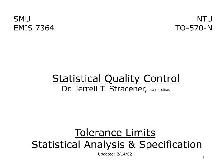
SMU EMIS 7364. NTU TO-570-N. Statistical Quality Control Dr. Jerrell T. Stracener, SAE Fellow. Tolerance Limits Statistical Analysis & Specification Updated: 2/14/02. Product Specification. Lower Specification Limit. Upper Specification Limit. Nominal Specification. x. Target

E N D
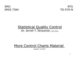
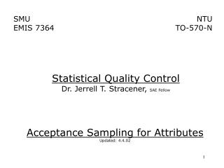
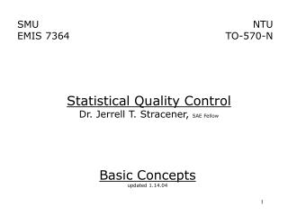
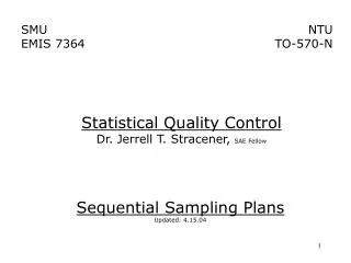
SMU EMIS 7364 NTU TO-570-N Statistical Quality Control Dr. Jerrell T. Stracener, SAE Fellow Tolerance Limits Statistical Analysis & Specification Updated: 2/14/02
Product Specification Lower Specification Limit Upper Specification Limit Nominal Specification x Target (Ideal level for use in product) Tolerance (Product characteristic) (Maximum range of variation of the product characteristic that will still work in the product.)
Traditional US Approach to Quality (Make it to specifications) No-Good No-Good Loss ($) good x LSL T USL
Variability Reduction • Variability reduction is a modern concept of design • and manufacturing excellence • Reducing variability around the target value leads • to better performing, more uniform, defect-free • product • Virtually eliminates rework and waste • Consistent with continuous improvement concept Don’t just conform to specifications Reduce variability around the target accept reject reject target
True Impact of Product Variability • Sources of loss • - scrap • - rework • - warranty obligations • - decline of reputation • - forfeiture of market share • Loss function - dollar loss due to deviation of • product from ideal characteristic • Loss characteristic is continuous - not a step • function.
Representative Loss Function Characteristics Loss $ Loss $ Loss $ x x x T X nominal is best L = k (x - T)2 X smaller is better L = k (x2) X larger is better L = k (1/x2)
Variability-Loss Relationship LSL USL Target Loss $ savings due to reduced variability Maximum $ loss per item
Loss Computation for Total Product Population X nominal is best L = k (x - T)2 Loss $ Loss $ x T x T
Statistical Tolerancing - Convention Normal Probability Distribution 0.00135 0.9973 0.00135 Nominal LTL UTL +3 -3
Statistical Tolerancing - Concept x LTL Nominal UTL
Caution For a normal distribution, the natural tolerance limits include 99.73% of the variable, or put another way, only 0.27% of the process output will fall outside the natural tolerance limits. Two points should be remembered: 1. 0.27% outside the natural tolerances sounds small, but this corresponds to 2700 nonconforming parts per million. 2. If the distribution of process output is non normal, then the percentage of output falling outside 3 may differ considerably from 0.27%.
Normal Distribution Probability Density Function: < x < where = 3.14159... e = 2.7183...
Normal Distribution • Mean or expected value of X • Mean = E(X) = • Median value of X • X0.5 = • Standard deviation
Normal Distribution Standard Normal Distribution If X ~ N(, ) and if , then Z ~ N(0, 1). A normal distribution with = 0 and = 1, is called the standard normal distribution.
Normal Distribution - example The diameter of a metal shaft used in a disk-drive unit is normally distributed with mean 0.2508 inches and standard deviation 0.0005 inches. The specifications on the shaft have been established as 0.2500 0.0015 inches. We wish to determine what fraction of the shafts produced conform to specifications.
f(x) 0.2500 nominal 0.2508 x 0.2485 LSL 0.2515 USL Normal Distribution - example solution
Normal Distribution - example solution Thus, we would expect the process yield to be approximately 91.92%; that is, about 91.92% of the shafts produced conform to specifications. Note that almost all of the nonconforming shafts are too large, because the process mean is located very near to the upper specification limit. Suppose we can recenter the manufacturing process, perhaps by adjusting the machine, so that the process mean is exactly equal to the nominal value of 0.2500. Then we have
Normal Distribution - example solution f(x) nominal 0.2485 LSL 0.2515 USL x 0.2500
What is the magnitude of the difference between sigma levels? Sigma Area Spelling Time Distance One Floor of 170 typos/page 31 years/century earth to moon Astrodome in a book Two Large supermarket 25 typos/page 4 years/century 1.5 times around in a book the earth Three small hardware 1.5 typos/page 3 months/century CA to NY store in a book Four Typical living 1 typo/30 pages 2 days/century Dallas to Fort Worth room ~(1 chapter) Five Size of the bottom 1 typo in a set of 30 minutes/century SMU to 75 Central of your telephone encyclopedias Six Size of a typical 1 typo in a 6 seconds/century four steps diamond small library Seven Point of a sewing 1 typo in several 1 eye-blink/century 1/8 inch needle large libraries
Linear Combination of Tolerances Xi = part characteristic for ith part, i = 1, 2, ... , n Xi ~ N(i, i) X1, X2, ..., Xn are independent
Linear Combination of Tolerances Y = assembly characteristic If , where the a1, ..., an are constants, then Y ~ N(Y, Y), where and
Concept x1 x2 . . . xn y
Statistical Tolerancing - Concept f(x) nominal x 0.2485 LSL 0.2515 USL 0.2500
Tolerance Analysis - example The mean external diameter of a shaft is S = 1.048 inches and the standard deviation is S = 0.0020 inches. The mean inside diameter of the mating bearing is b = 1.059 inches and the standard deviation is b = 0.0030 inches. Assume that both diameters are normally and independently distributed. (a) What is the required clearance, C, such that the probability of an assembly having a clearance less than C is 1/1000? (b) What is the probability of interference?
Bearing Xb Shaft XS Tolerance Analysis - example solution fb(x) fs(x)
Tolerance Analysis - example solution Intersection Region fb(x) fs(x)
The Normal Model - example solution D = xb-xs = Clearance of bearing inside diameter minus shaft outside diameter D = b - S = 0.011 D = (b2 + S2)1/2 = 0.0036 so D~N(0.011,0.0036) fD(x) d=xb-xs
The Normal Model - example solution (a) Find c such that P(D < c) = so that From the normal table (found in the resource section of the website), the Z = -3.09 so that and
The Normal Model - example solution Since c < 0, there is no value of c for which the probability is equal to 0.001 (b) Find the probability of interference, i.e., From the normal table (found in the resource section of the website), the Z of -3.1 = 0.0011
Tolerance Analysis - example Using Monte Carlo Simulation (n=1000): (a) What is the required clearance, C, such that the probability of an assembly having a clearance less than C is 1/1000? (b) What is the probability of interference?
Tolerance Analysis - example Using Monte Carlo Simulation First generate random samples from (I used n=1000) Xbi~N(mb, sb) = N(1.059, 0.0030) and Xsi~N(ms, ss) = N(1.048, 0.0020)
Tolerance Analysis - example Then calculate the differences Estimate Estimate ms by taking the mean. (You can use the AVERAGE() function.) Estimate ss by calculating the standard deviation.(You can use the STDEV() function.)
Tolerance Analysis - example =0.01093 and =0.00371 (a) This is close to c = -0.000124.
Tolerance Analysis - example (b) This can be compared to P(I) = 0.000968.
Statistical Tolerance Analysis Process • Assembly consists of K components • Specifications Assembly: • Specifications Component: • Assembly Nominal • where ai = 1 or -1 as appropriate
Statistical Tolerance Analysis Process • Assembly tolerance • If dimension • with parameters and , then • where • and
Statistical Tolerance Analysis Process • is specified • is determined during design • is calculated • Case 1: if probability is too small, then • (1) component tolerance(s) must be reduced • or (2) tA must be increased
Statistical Tolerance Analysis Process Case 2: if probability is too large, then some or all components tolerances must be increased. Note: Do not perform a worst-case tolerance analysis
Tolerance Limits Based on the Normal Distribution Suppose a random variable x is distributed with mean m and variance s2, both unknown. From a random sample of n observations, the sample mean and sample variance S2 may be computed. A logical procedure for estimating the natural tolerance limits m ± Za/2 s is to replace m by and s by S, yielding.
Tolerance Intervals - Two-Sided Since and S are only estimates and not the true parameters values, we cannot say that the above interval always contains 100(1 - a)% of the distribution. However, one may determine a constant K, such that in a large number of samples a faction
Tolerance Intervals - Two-Sided If X1, X2, …, Xn is a random sample of size n from a normal distribution with unknown mean and unknown standard deviation , then a two-sided tolerance interval is (LTL,UTL), i.e., an interval that contains at least the proportion P of the population, with g 100% confidence is: and is a function of n, P, and g and may be obtained from the table Factors for Two-Sided Tolerance Limits for Normal Distributions (Located in the resource section on the website).
Tolerance Intervals - One-Sided If X1, X2, …, Xn is a random sample of size n from a normal distribution with unknown mean and unknown standard deviation , then a one-sided lower (upper) tolerance interval is defined by the lower tolerance limit LTL (upper tolerance limit UTL), the value for which at least the proportion P of the population lies above (below) LTL (UTL) with g100% confidence where is a function of n, P, and g and may be obtained from the table Factors for Once-Sided Tolerance Limits for Normal Distributions (Located in the resource section on the website).
Tolerance Intervals - Two-Sided Example Ten washers are selected at random from a population that can be described by a normal distribution. The measured thicknesses, in inches, are: Establish an interval that contains at least 90% of the population of washer thicknesses with 95% confidence.
Tolerance Intervals - Two-Sided Example Solution From the sample data and The K value can be found on Tolerance Limits Table- Two-Sided with gamma 95 and 99 and n=2 to 27(Located in the resource section on the website).
Tolerance Intervals - Two-Sided Example Solution so that Therefore, with 95% confidence at least 90% of the population of washer thicknesses, in inches, will be contained in the interval (0.116,0.136).