Objectives: Review MAP Derivation

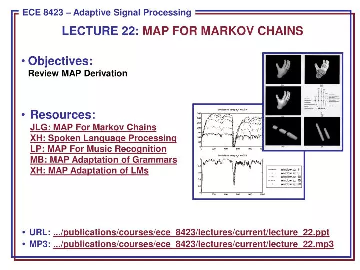
1. LECTURE 22: MAP FOR MARKOV CHAINS • Objectives:Review MAP Derivation • Resources:JLG: MAP For Markov ChainsXH: Spoken Language ProcessingLP: MAP For Music RecognitionMB: MAP Adaptation of GrammarsXH: MAP Adaptation of LMs • URL: .../publications/courses/ece_8423/lectures/current/lecture_22.ppt • MP3: .../publications/courses/ece_8423/lectures/current/lecture_22.mp3

2. Introduction • Consider the problem of estimating  given a sequence of observations, o. The maximum a posteriori (MAP) estimate of  is given by: • Three key issues need to be addressed: the choice of the prior distribution family, the specification of the parameters for the prior densities, and the evaluation of the MAP. • These problems are closely related since an appropriate choice of the prior distribution can greatly simplify the MAP estimation process. • For both finite mixture densities and hidden Markov models, EM must be used because the distribution lacks a sufficient statistic due to the underlying hidden process (i.e., the state mixture component and the state sequence of a Markov chain for an HMM). • For HMM parameter estimation, EM is known as the Baum-Welch (BW) algorithm and alternates between maximizing the likelihood function of the observed data and reestimating the parameters using expectations. • We will assume the data is generated from a multivariate Gaussian distribution, and the T observations are i.i.d. and independent. • We will ignore the use of mixture densities (see Gauvain, 1994 for the details).

3. The Likelihood Function • The likelihood of the data (with respect to the kth state) can be written as: • The matrix r is referred to as the precision matrix and is defined as the inverse of the covariance matrix. The constant terms in the Gaussian are ignored because they don’t affect the optimization. • The prior distribution for the Gaussian mean and covariance is approximated with a normal-Wishart distribution: • A Wishart distribution is a multidimensional generalization of the Chi-squared distribution. A Chi-squared distribution results from taking the sum of the squares of Gaussian random variables. • The vector and matrix, , are the prior density parameters for . • : number of degrees of freedom; : proportional to the prior prob.

4. MAP Estimates for a Gaussian • The EM algorithm can be applied to find the ML estimates. The auxiliary function, , that is maximized is the combination of: • The auxiliary function, , is given by: • Continue from the Gauvain paper.