Download
1 / 16
160 likes | 330 Views
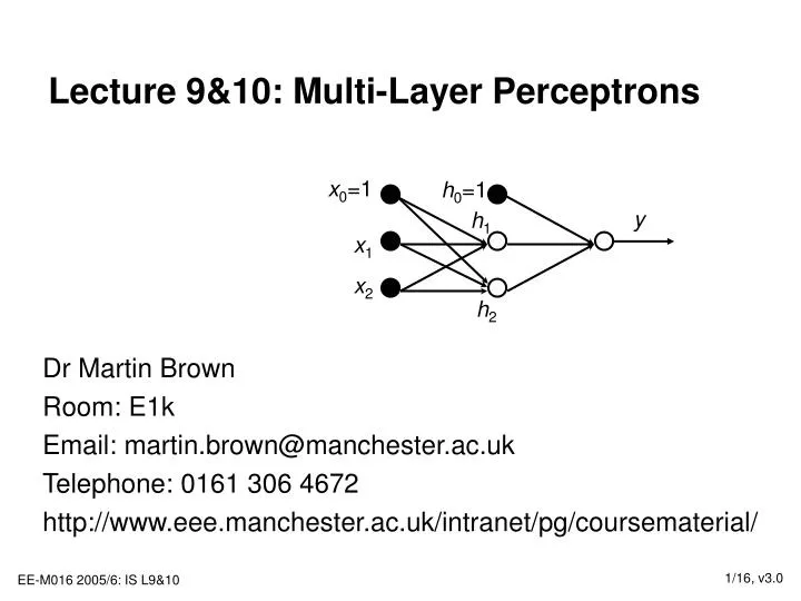
Lecture 9&10: Multi-Layer Perceptrons. x 0 =1. h 0 =1. y. h 1. x 1. x 2. h 2. Dr Martin Brown Room: E1k Email: martin.brown@manchester.ac.uk Telephone: 0161 306 4672 http://www.eee.manchester.ac.uk/intranet/pg/coursematerial/. Lecture 9&10: Outline.

E N D
Lecture 9&10: Multi-Layer Perceptrons x0=1 h0=1 y h1 x1 x2 h2 Dr Martin Brown Room: E1k Email: martin.brown@manchester.ac.uk Telephone: 0161 306 4672 http://www.eee.manchester.ac.uk/intranet/pg/coursematerial/
Lecture 9&10: Outline • Layered sigmoidal models (multi-layer perceptrons – MLP) • Network structure and modelling abilities • Gradient descent for MLPs (error back propagation – EBP) • Example: learning XOR solution • Variations on/extensions to basic, non-linear gradient descent parameter estimation • MLPs are non-linear in both: • Inputs/features, therefore the models for non-linear decision boundaries and non-linear regression surfaces • Parameters, therefore gradient descent can only be used to show convergence to a local minimum
Lecture 9&10: Resources • These slides are largely self-contained, but extra, background material can be found in: • Machine Learning, T Mitchell, McGraw Hill, 1997 • Machine Learning, Neural and Statistical Classification, D Michie, DJ Spiegelhalter and CC Taylor, 1994: http://www.amsta.leeds.ac.uk/~charles/statlog/ • In addition, there are many on-line sources for multi-layer perceptrons (MLPs) and error back propagation (EBP), just search on google • Advanced text: • Information Theory, Inference and Learning Algorithms, D MacKay, Cambridge University Press, 2003
Multi-Layer Perceptron Networks • Layered perceptron (with bi-polar/binary outputs) networks can realize any logical function, however there is no simple way to estimate the parameters/generalise the (single layer) Perceptron convergence procedure • Multi-layer perceptron (MLP) networks are a class of models that are formed from layered sigmoidal nodes, which can be used for regression or classification purposes. • They are commonly trained using gradient descent on a mean squared error performance function, using a technique known as error back propagation in order to calculate the gradients. • Widely applied to many prediction and classification problems over the past 15 years.
Multi-Layer Perceptron Networks • Use 2 or more layers of parameters where: • Empty circles represent sigmoidal (tanh) nodes • Solid circles represent real signals (inputs, biases & outputs) • Arrows represent adjustable parameters • Multi-Layer Perceptron networks can have: • Any number of layers of parameters (but generally just 2) • Any number of outputs (but generally just 1) • Any number of nodes in the hidden layers (see Slide 14) x0=1 h0=1 y h1 x1 x2 Output layer qo h2 Hidden layer Qh
Exemplar Model Outputs MLP with two hidden nodes. The response surface resembles an “impulse ridge” because one sigmoid is subtracted from the other. This is a learnt solution to the “classification” XOR problem. This non-linear regression surface is generated by an MLP with three hidden nodes, and a linear transfer function in the output layer
^ ^ qk qk+1 Gradient Descent Parameter Estimation • All of the model’s parameters can be stacked up into a single vector q, then use gradient descent learning: • q0 are small, random values • Performance function(s) non-linear in q • No direct solution • Local minima are possible • Learning rate is difficult to estimate because local Hessian (second derivative matrix) varies in parameter space ^ p ^ q q
Output Layer Gradient Calculation Hidden layer Output layer … Gradient descent update: For the ith training pattern: Using the chain rule: Giving an update rule: Same as the derivation for a single-layer sigmoidal model, as described in lecture 7&8.
x S f() Hidden Layer Gradient Calculation Analyze the path such that altering the jth hidden node’s parameter vector affects the model’s output By the chain rule: Gradient expression (back error propagation):
MLP Iterative Parameter Estimation • Randomly initialise all parameters in network (to small values) • For each parameter update • present each input pattern to the network & get output • calculate the update for each parameter according to: • where: • output layer • hidden layer • calculate average parameter updates • update weights • Stop when steps > max_steps or MSE < tolerance or test MSE is minimum
Example: Learning the XOR Problem Performance history for the XOR data and MLP with 2 hidden nodes. Note its non-monotonic behaviour, also large number of iterations h = 0.05, update after each datum Learning histories for the 9 parameters in the MLP. Note that even when the MSE goes up, the parameters are heading towards “optimal” values
Example: Trained XOR Model • The trained optimal model has a ridge where the target is 1 and plateaus out in the regions where target is –1. Note all inputs and targets are bipolar {–1,1}, rather than binary
Basic Variations on Parameter Estimation • Parameter updates can be performed: • After each pattern is presented (LMS) • After the complete data set has been presented (Batch) • Generally, convergence is smoother in the latter case, though overall convergence may be slower • When to stop learning is typically done by monitoring the performance and stopping when an acceptable level is reached, before the parameters become too large. • Learning rate needs to be carefully selected to ensure stable learning along the parameter trajectory within a reasonable time period • Generally, input features are scaled to zero mean, unit variance (or lie between [–1, 1])
. Validation (final performance) performance Testing (model selection) Training (parameter estimation) number of hidden nodes Selecting the Size of the Hidden Layer • In building a non-linear model such as an MLP, the labelled data may be divided into 3 sets • Training: used to learn the optimal parameters values • Testing: used to compare different model structures • Validation: used to get a final performance figures • The aim is to select a model that performs well on the test set, and use the validation set to obtain a final performance estimate. • Use to select number of nodes in hidden layer
Lecture 9&10: Conclusions • Multi-layer perceptrons are universal approximators – they can model any continuous function arbitrarily closely, given sufficient number of hidden nodes (existence proof only) • Used for both classification and regression problems, although with regression, often a linear transfer function is used in the output layer so that the output is unbounded. • Trained using gradient descent, which suffers all the well-known disadvantages. • Sometimes known as “error back propagation” because the output error is fed backwards to the gradient signal of the hidden layer(s). • The number of hidden nodes, and learning rate, needs to be experimentally found, often using separate training, testing and validation data sets
Lecture 9&10: Laboratory Session • Make sure you have the Single Layer Sigmoid, trained using gradient descent, algorithm working (see lab 7&8). This forms the main part of your assignment. • Extend this procedure to implement an MLP to solve the XOR problem. You should note that the output layer is equivalent to an single layer sigmoid, and that all you have to add is the output and parameter update calculations for the hidden layer. • Make sure this works by monitoring the MSE and showing that it tends to 0 as the number of iterations increases – you’ll need two hidden nodes • Draw the logical function boundaries for each node to verify that the output is correct.