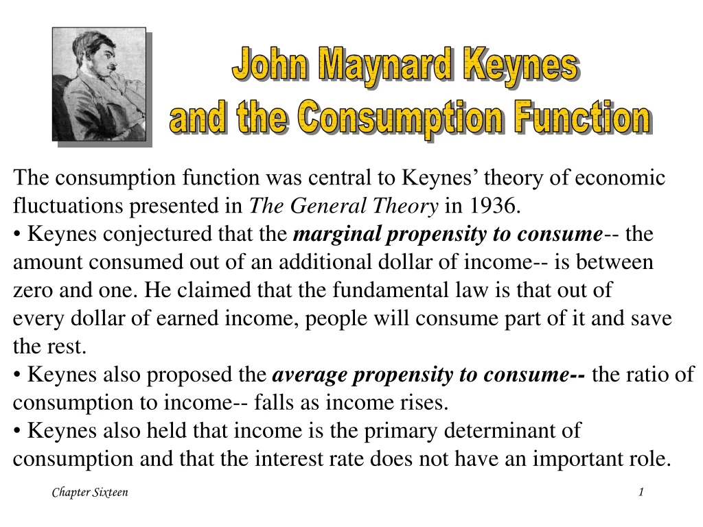
John Maynard Keynes and the Consumption Function

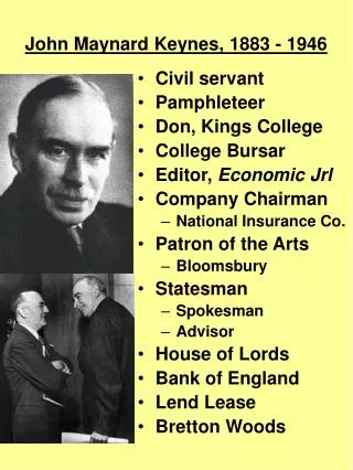
1. John Maynard Keynes and the Consumption Function • The consumption function was central to Keynes’ theory of economic • fluctuations presented in The General Theory in 1936. • Keynes conjectured that the marginal propensity to consume-- the amount consumed out of an additional dollar of income-- is between • zero and one. He claimed that the fundamental law is that out of • every dollar of earned income, people will consume part of it and save • the rest. • Keynes also proposed the average propensity to consume-- the ratio of consumption to income-- falls as income rises. • Keynes also held that income is the primary determinant of consumption and that the interest rate does not have an important role.

2. Example from development economies in practise • Do the law of one price holds? • Example from Pizza Hut in Russia. • Property rights in Russia. • Can the nominal interest rate be negative? (Risk of burglary.) • Do government renege on debt. • Government bonds in terms of cars. • Can economist make forecasts? • Ex. from Asian Development Bank

3. What is mercantilism? • Should a country who • Cares about consumtion increase exports • And there by accumulate wealth? • When news papers say exports are up, • It is considered to be something good. • Under what condition (s)?

4. C C = C + cY C = C + cY consumption spending by households income Marginal Propensity to consume (MPC) depends on C Y Autonomous consumption The slope of the consumption function is the MPC. The Consumption Function

5. APC = C/Y = C/Y + c The Average Propensity to Consume This consumption function exhibits three properties that Keynes conjectured. First, the marginal propensity to consume c is between zero and one. Second, the average propensity to consume falls as income rises. Third, consumption is determined by current income. C APC1 C APC2 1 1 Y As Y rises, C/Y falls, and so the average propensity to consume C/Y falls. Notice that the interest rate is not included in this function.

6. Secular Stagnation, Simon Kuznets, and the Consumption Puzzle During World War II, on the basis of Keynes’ consumption function, economists predicted that the economy would experience what they called secular stagnation-- a long depression of infinite duration-- unless fiscal policy was used to stimulate aggregate demand. It turned out that the end of the war did not throw the U.S. into another depression, but it did suggest that Keynes’ conjecture that the average propensity to consume would fall as income rose appeared not to hold. Simon Kuznets constructed new aggregate data on consumption and investment dating back to 1869 and whose work would later earn a Nobel Prize. He discovered that the ratio of consumption to income was stable over time, despite large increases in income; again, Keynes’ conjecture was called into question. This brings us to the puzzle…

7. Consumption Puzzle The failure of the secular-stagnation hypothesis and the findings of Kuznets both indicated that the average propensity to consume is fairly constant over time. This presented a puzzle: why did Keynes’ conjectures hold up well in the studies of household data and in the studies of short time-series, but fail when long time series were examined? Studies of household data and short time-series found a relationship between consumption and income similar to the one Keynes conjectured-- this is called the short-run consumption function. But, studies using long time-series found that the APC did not vary systematically with income--this relationship is called the long-run consumption function. Long-run consumption function (constant APC) C Short-run consumption function (falling APC) Y

8. Irving Fisher and Intertemporal Choice The economist Irving Fisher developed the model with which economists analyze how rational, forward-looking consumers make intertemporal choices-- that is, choices involving different periods of time. The model illuminates the constraints consumers face, the preferences they have, and how these constraints and preferences together determine their choices about consumption and saving. When consumers are deciding how much to consume today versus how much to consume in the future, they face an intertemporal budget constraint, which measures the total resources available for consumption today and in the future.

9. Fischer’s life-cycle model: individual lives 2 periods, no uncertainty. Period 1 constraint: S=Y1-C1 Period 2 constraint: C2=(1+r)S+Y2 Inserting (1) into (2) gives the intertemporal budget constraint: C2=(1+r)(Y1-C1)+Y2  C1+C2/(1+r) = Y1 + Y2/(1+r) This intertemporal consumer’s budget constraint implies that if the interest rate is zero, the budget constraint shows that total consumption in the two periods equals total income in the two periods. In the usual case in which the interest rate is greater than zero, future consumption and future income are discounted by a factor of 1 + r. This discounting arises from the interest earned on savings. Because the consumer earns interest on current income that is saved, future income is worth less than current income.  C2 = (1+r)*Y1 + Y2 – (1+r)*C1

10. The Consumer's Budget Constraint Here are the combinations of first-period and second-period consumption the consumer can choose. If he chooses a point between A and B, he consumes less than his income in the first period and saves the rest for the second period. If he chooses between A and C, he consumes more that his income in the first period and borrows to make up the difference. Consumer’s budget constraint Second- period consumption B Saving Vertical intercept is (1+r)Y1 + Y2 A Borrowing Y2 Horizontal intercept is Y1 + Y2/(1+r) C Y1 First-period consumption

11. Consumer Preferences Second- period consumption Y Z IC2 X IC1 W First-period consumption Indifference curves represent the consumer’s preferences over first- period and second-period consumption. An indifference curve gives the combinations of consumption in the two periods that make the consumer equally happy. Higher indifferences curves such as IC2 are preferred to lower ones such as IC1. The consumer is equally happy at points W, X, and Y, but prefers Z to all the others-- Point Z is on a higher indifference curve and is therefore not equally preferred to W, X and Y.

12. Optimization Second- period consumption O IC3 IC2 IC1 First-period consumption The consumer achieves his highest (or optimal) level of satisfaction by choosing the point on the budget constraint that is on the highest indifference curve. At the optimum, the indifference curve is tangent to the budget constraint.

13. How Changes in Income Affect Consumption Second- period consumption O IC2 IC1 First-period consumption An increase in either first-period income or second-period income shifts the budget constraint outward. If consumption in period one and consumption in period two are both normal goods-- those that are demanded more as income rises, this increase in income raises consumption in both periods.

14. How Changes in the Real Interest Rate Affect Consumption Economists decompose the impact of an increase in the real interest rate on consumption into two effects: an income effect and a substitution effect. The income effect is the change in consumption that results from the movement to a higher indifference curve. The substitution effect is the change in consumption that results from the change in the relative price of consumption in the two periods. An increase in the interest rate rotates the budget constraint around the point C, where C is (Y1, Y2). The higher interest rate reduces first period consumption (move to point A) and raises second-period consumption (move to point B). In this figure. New budget constraint Second- period consumption B Old budget constraint A C Y2 IC2 IC1 Y1 First-period consumption

15. Franco Modigliani and the Life-Cycle Hypothesis In the 1950’s, Franco Modigliani, Ando and Brumberg used Fisher’s model of consumer behavior to study the consumption function. One of their goals was to study the consumption puzzle. According to Fisher’s model, consumption depends on a person’s lifetime income: C1=f(life-time income: Y1+Y2/(1+r) ), C2=h(Y1+Y2/(1+r) ) An increase in income is spread out over both periods of life: Consumers want a smooth consumption pattern when income varies. An increase in Y1 increases both C1 and C2 (by increased S). An increase in Y2 increases both C1 (through less saving) and C2. Modigliani emphasized that income varies systematically over people’s lives and that saving allows consumers to move income from those times in life when income is high to those times when income is low. This interpretation of consumer behavior formed the basis of his life-cycle hypothesis: Implication: Income varies more than consumption.

16. Milton Friedman and the Permanent-Income Hypothesis In 1957, Milton Friedman proposed the permanent-income hypothesis to explain consumer behavior. Its essence is that current consumption is proportional to permanent income. Friedman’s permanent-income hypothesis complements Modigliani’s life-cycle hypothesis: both use Fisher’s theory of the consumer to argue that consumption should not depend on current income alone. But unlike the life-cycle hypothesis, which emphasizes that income follows a regular pattern over a person’s lifetime, the permanent-income hypothesis emphasizes that people experience random and temporary changes in their incomes from year to year. Friedman suggested that we view current income Y as the sum of two components, permanent income YPand transitory income YT.

17. Fischer’s model and the trade balance Assume that all individuals are identical, no uncertainty, no initial foreign debt. Applying the life-cycle model to a country. (However, a country lives on longer as well as do families). • (1) Export=Y1-C1, when exports are negative we import. • (2) C2=(1+r)Export+Y2 • Inserting (1) into (2) gives: C2=(1+r)(Y1-C1)+Y2 •  C1+C2/(1+r) = Y1 + Y2/(1+r) Just to simplify (absolutely not necessary assumption): Assume to start with that C1=Y1 and C2=Y2 → Exports=0 → imports = 0. Ex.1: Y1 ↓→ C1 ↓ and C2 ↓. C1 falls less than Y1 because of consumption smoothing → country borrows/imports in period 1 C2 falls while Y2 unchanged means the country exports in period 2 To pay off its foreign debt. Over the 2 periods trade balance is 0 in PDV. Ex.2 Y1 ↑ → C1 ↑ and C2 ↑. C2 can only increase if saving = exports in period 1 ↑. Ex.3 Y2 ↑ → C1 ↑ and C2 ↑. Country imports in period 1.

18. Constraints on Borrowing The inability to borrow prevents current consumption from exceeding current income. A constraint on borrowing can therefore be expressed as C1 < Y1. This inequality states that consumption in period one must be less than or equal to income in period one. This additional constraint on the consumer is called a borrowing constraint, or sometimes, a liquidity constraint. The analysis of borrowing leads us to conclude that there are two consumption functions. For some consumers, the borrowing constraint is not binding, and consumption in both periods depends on the present value of lifetime income. For other consumers, the borrowing constraint binds. Hence, for those consumers who would like to borrow but cannot, consumption depends only on current income.

19. David Laibson and the Pull of Instant Gratification Recently, economists have turned to psychology for further explanations of consumer behavior. They have suggested that consumption decisions are not made completely rationally. Laibson notes that many consumers judge themselves to be imperfect decision-makers. Consumers’ preferences may be time-inconsistent: they may alter their decisions simply because time passes. Pull of Instant Gratification