Download
1 / 19
200 likes | 326 Views
Splines and Piecewise Interpolation. Berlin Chen Department of Computer Science & Information Engineering National Taiwan Normal University. Reference: 1. Applied Numerical Methods with MATLAB for Engineers , Chapter 18 & Teaching material. Chapter Objectives (1/2).

E N D
Splines and Piecewise Interpolation Berlin Chen Department of Computer Science & Information Engineering National Taiwan Normal University Reference: 1. Applied Numerical Methods with MATLAB for Engineers, Chapter 18 & Teaching material
Chapter Objectives (1/2) • Understanding that splines minimize oscillations by fitting lower-order polynomials to data in a piecewise fashion • Knowing how to develop code to perform table lookup • Recognizing why cubic polynomials are preferable to quadratic and higher-order splines • Understanding the conditions that underlie a cubic fit • Understanding the differences between natural, clamped, and not-a-knot end conditions
Chapter Objectives (2/2) • Knowing how to fit a spline to data with MATLAB’s built-in functions • Understanding how multidimensional interpolation is implemented with MATLAB
Introduction to Splines • An alternative approach to using a single (n-1)th order polynomial to interpolate between n points is to apply lower-order polynomials in a piecewise fashion to subsets of data points • These connecting polynomials are called spline functions • Splines minimize oscillations and reduce round-off error due to their lower-order nature
Higher-Order Polynomials vs. Splines • Splines eliminate oscillations by using small subsets of points for each interval rather than every point. This is especially useful when there are jumps in the data: • 3rd order polynomial • 5th order polynomial • 7th order polynomial • Linear spline - Seven 1st order polynomials generated by using pairs of points at a time
Spline Development (1/2) • Spline function (si(x)) coefficients are calculated for each interval of a data set • The number of data points (fi) used for each spline function depends on the order of the spline function
Spline Development (2/2) • First-order splines find straight-lineequations between each pair of points that • Go through the points • Second-order splines find quadratic equations between each pair of points that • Go through the points • Match first derivatives at the interior points • Third-order splines find cubic equations between each pair of points that • Go through the points • Match first and second derivatives at the interior pointsNote that the results of cubic spline interpolation are different from the results of an interpolating cubic.
Cubic Splines (1/2) • While data of a particular size presents many options for the order of spline functions, cubic splines are preferred because they provide the simplest representation that exhibits the desired appearance of smoothness • Linear splines have discontinuous first derivatives • Quadratic splines have discontinuous second derivatives and require setting the second derivative at some point to a pre-determined value*but* • Quartic or higher-order splines tend to exhibit the instabilities inherent in higher order polynomials (ill-conditioning or oscillations)
Cubic Splines (2/2) • In general, the ith spline function for a cubic spline can be written as: • For n data points, there are n-1 intervals and thus 4(n-1) unknowns to evaluate to solve all the spline function coefficients
Solving Cubic Spline Coefficients • One condition requires that the spline function goes through the first and last point of the interval, yielding 2(n-1) equations of the form: • Another requires that the first derivative is continuous at each interior point, yielding n-2 equations of the form: • A third requires that the second derivative is continuous at each interior point, yielding n-2 equations of the form: • These give 4n-6 total equations and 4n-4 are needed!
Two Additional Equations for Cubic Splines • There are several options for the final two equations: • Natural end conditions - assume the second derivative at the end knots are zero • Clamped end conditions - assume the first derivatives at the first and last knots are known • “Not-a-knot” end conditions - force continuity of the third derivative at the second and penultimate (next-to-last) points • Result in the first two intervals having the same spline function and the last two intervals having the same spline function
Piecewise Interpolation in MATLAB • MATLAB has several built-in functions to implement piecewise interpolation. The first is spline: yy=spline(x, y, xx) This performs cubic spline interpolation, generally using not-a-knot conditions. If y contains two more values than x has entries, then the first and last value in y are used as the derivatives at the end points (i.e. clamped)
Not-a-knot Example • Generate data:x = linspace(-1, 1, 9);y = 1./(1+25*x.^2); • Calculate 100 model points anddetermine not-a-knot interpolationxx = linspace(-1, 1);yy = spline(x, y, xx); • Calculate actual function values at model points and data points, the 9-point not-a-knot interpolation (solid), and the actual function (dashed), yr = 1./(1+25*xx.^2)plot(x, y, ‘o’, xx, yy, ‘-’, xx, yr, ‘--’)
Clamped Example • Generate data w/ first derivative information:x = linspace(-1, 1, 9);y = 1./(1+25*x.^2);yc = [1 y -4] %(specified slops at boundaries) • Calculate 100 model points anddetermine clamped interpolationxx = linspace(-1, 1);yyc = spline(x, yc, xx); • Calculate actual function values at model points and data points, the 9-point clamped interpolation (solid), and the actual function (dashed), yr = 1./(1+25*xx.^2)plot(x, y, ‘o’, xx, yyc, ‘-’, xx, yr, ‘--’) The clamped spline exhibits some oscillations because of the artificial slops being imposed at the boundaries.
MATLAB’s interp1 Function • While spline can only perform cubic splines, MATLAB’s interp1 function can perform several different kinds of interpolation:yi = interp1(x, y, xi, ‘method’) • x & y contain the original data • xi contains the points at which to interpolate • ‘method’ is a string containing the desired method: • ‘nearest’ - nearest neighbor interpolation • ‘linear’ - connects the points with straight lines • ‘spline’ - not-a-knot cubic spline interpolation • ‘pchip’ or ‘cubic’ - piecewise cubic Hermite interpolation (the second derivatives are not necessarily continuous)
Multidimensional Interpolation (1/2) • The interpolation methods for one-dimensional problems can be extended to multidimensional interpolation. • Example - bilinear interpolationusing Lagrange-form equations
Multidimensional Interpolation (2/2) • First hold the y value fixed • Then, linearly interpolate along the y dimension • Finally we can arrive at
Multidimensional Interpolation in MATLAB • MATLAB has built-in functions for two- and three-dimensional piecewise interpolation: zi = interp2(x, y, z, xi, yi, ‘method’) vi = interp3(x, y, z, v, xi, yi, zi, ‘method’) • ‘method’ is again a string containing the desired method: ‘nearest’, ‘linear’, ‘spline’,‘pchip’, or ‘cubic’ • For 2-D interpolation, the inputs must either be vectors or same-size matrices • For 3-D interpolation, the inputs must either be vectors or same-size 3-D arrays