Physical Mapping – Restriction Mapping

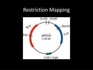
Physical Mapping – Restriction Mapping

Molecular Scissors Molecular Cell Biology, 4th edition

Discovering Restriction Enzymes • HindII - first restriction enzyme – was discovered accidentally in 1970 while studying how the bacterium Haemophilus influenzae takes up DNA from the virus • Recognizes and cuts DNA at sequences: • GTGCAC • GTTAAC

Discovering Restriction Enzymes My father has discovered a servant who serves as a pair of scissors. If a foreign king invades a bacterium, this servant can cut him in small fragments, but he does not do any harm to his own king. Clever people use the servant with the scissors to find out the secrets of the kings. For this reason my father received the Nobel Prize for the discovery of the servant with the scissors". Daniel Nathans’ daughter (from Nobel lecture) Werner Arber Daniel NathansHamilton Smith Werner Arber – discovered restriction enzymes Daniel Nathans - pioneered the application of restriction for the construction of genetic maps Hamilton Smith - showed that restriction enzyme cuts DNA in the middle of a specific sequence

Recognition Sites of Restriction Enzymes Molecular Cell Biology, 4th edition

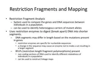
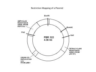
Restriction Maps • A map showing positions of restriction sites in a DNA sequence • If DNA sequence is known then construction of restriction map is a trivial exercise • In early days of molecular biology DNA sequences were often unknown • Biologists had to solve the problem of constructing restriction maps without knowing DNA sequences

Physical map • Definition:Let S be a DNA sequence. A physical mapconsists of a set M of markers and afunction p : M Nthat assigns each marker a position of M in S. • N denotes the set of nonnegative integers

Restriction mapping problem • For a set X of points on the line, let DX = {| x1 - x2| : x1, x2  X}denote the multisetof all pairwise distances between points in X. In the restriction mapping problem, asubset E DX (of experimentally obtained fragment lengths) is given and the task is toreconstruct X from E.

Full Restriction Digest • DNA at each restriction site creates multiple restriction fragments: Is it possible to reconstruct the order of the fragments from the sizes of the fragments {3,5,5,9} ?

Full Restriction Digest: Multiple Solutions • Alternative ordering of restriction fragments: vs

Measuring Length of Restriction Fragments • Restriction enzymes break DNA into restriction fragments. • Gel electrophoresis is a process for separating DNA by size and measuring sizes of restriction fragments • Can separate DNA fragments that differ in length in only 1 nucleotide for fragments up to 500 nucleotides long

Gel Electrophoresis • DNA fragments are injected into a gel positioned in an electric field • DNA are negatively charged near neutral pH • The ribose phosphate backbone of each nucleotide is acidic; DNA has an overall negative charge • DNA molecules move towards the positive electrode • DNA fragments of different lengths are separated according to size • Smaller molecules move through the gel matrix more readily than larger molecules • The gel matrix restricts random diffusion so molecules of different lengths separate into different bands

Gel Electrophoresis: Example Direction of DNA movement Smaller fragments travel farther Molecular Cell Biology, 4th edition

Vizualization of DNA:Autoradiography and Fluorescence • autoradiography: • The DNA is radioactively labeled. The gel is laid against a sheet of photographic film in the dark, exposing the film at the positions where the DNA is present • fluorescence: • The gel is incubated with a solution containing the fluorescent dye ethidium – ethidium binds to the DNA • The DNA lights up when the gel is exposed to ultraviolet light.

Three different problems • the double digest problem – DDP • the partial digest problem – PDP • the simplified partial digest problem – SPDP

Double Digest Mapping • Use two restriction enzymes; three full digests: • a complete digest ofSusing A, • a complete digest ofSusing B, and • a complete digest ofSusing bothAandB. • Computationally, Double Digest problem is more complex than Partial Digest problem

Double Digest: Example

Double Digest: Example Without the information about X (i.e.A+B), it is impossible to solve the double digest problem as this diagram illustrates

Double Digest Problem Input: dA – fragment lengths from the complete digest with enzyme A. dB – fragment lengths from the complete digest with enzyme B. dX – fragment lengths from the complete digest with bothA and B. Output: A– location of the cuts in the restriction map for the enzyme A. B – location of the cuts in the restriction map for the enzyme B.

Double Digest: Multiple Solutions

Double digest • The decision problem of the DDP is NP-complete. • All algorithms have problems with more than 10 restriction sites for each enzyme. • A solution may not be unique and the number of solutions grows exponenially. • DDP is a favorite mapping method since the experiments are easy to conduct.

DDP is NP-complete • Is in NP – easy • given a set of integers X = {x1, . . . , xl}. The Set Partitioning Problem (SPP) is to determinewhether we can partition Xin into two subsets X1 and X2 such that • This problemis known to be NP-complete.

DDP is NP-complete • Let Xbe the input of the SPP, assuming that the sum of all elements of Xis even. Then set • dA = X, • dB =. with , and • dAB = dA. • then there exists an index n0 with because of the choice of DB and DAB. Thus a solution for the SPP exists. • thus SPP is a DDP in which one of the two enzymes produced only two fragments of equal length.

Partial Restriction Digest • The sample of DNA is exposed to the restriction enzyme for only a limited amount of time to prevent it from being cut at all restriction sites • This experiment generates the set of all possible restriction fragments between every two (not necessarily consecutive) cuts • This set of fragment sizes is used to determine the positions of the restriction sites in the DNA sequence

Multiset of Restriction Fragments • We assume that multiplicity of a fragment can be detected, i.e., the number of restriction fragments of the same length can be determined (e.g., by observing twice as much fluorescence intensity for a double fragment than for a single fragment) Multiset: {3, 5, 5, 8, 9, 14, 14, 17, 19, 22}

Partial Digest Fundamentals the set of n integers representing the location of all cuts in the restriction map, including the start and end X: n: the total number of cuts DX: the multiset of integers representing lengths of each of the fragments produced from a partial digest

One More Partial Digest Example Representation of DX= {2, 2, 3, 3, 4, 5, 6, 7, 8, 10} as a two dimensional table, with elements of X = {0, 2, 4, 7, 10} along both the top and left side. The elements at (i, j) in the table is xj – xi for 1 ≤ i < j ≤ n.

Partial Digest Problem: Formulation Goal: Givenall pairwise distances between points on a line, reconstruct the positions of those points • Input: The multiset of pairwise distances L, containing n(n-1)/2integers • Output: A set X, of n integers, such that DX = L

Partial Digest: Multiple Solutions • It is not always possible to uniquely reconstruct a set X based only on DX. • For example, the set X = {0, 2, 5} and (X+ 10) = {10, 12, 15} both produce DX={2, 3, 5} as their partial digest set. • The sets {0,1,2,5,7,9,12} and {0,1,5,7,8,10,12} present a less trivial example of non-uniqueness. They both digest into: {1, 1, 2, 2, 2, 3, 3, 4, 4, 5, 5, 5, 6, 7, 7, 7, 8, 9, 10, 11, 12}

Homometric Sets

Partial Digest: Brute Force • Find the restriction fragment of maximum length M. M is the length of the DNA sequence. • For every possible set X={0, x2, … ,xn-1, M} compute the corresponding DX • If DX is equal to the experimental partial digest L, then X is the correct restriction map

BruteForcePDP • BruteForcePDP(L, n): • M maximum element in L • for every set of n – 2 integers 0 < x2 < … xn-1 < M • X {0,x2,…,xn-1,M} • Form DX from X • if DX = L • return X • output “no solution”

Efficiency of BruteForcePDP • BruteForcePDP takes O(Mn-2) time since it must examine all possible sets of positions. • One way to improve the algorithm is to limit the values of xi to only those values which occur in L.

AnotherBruteForcePDP • AnotherBruteForcePDP(L, n) • M maximum element in L • for every set of n – 2 integers 0 < x2 < … xn-1 < M • X { 0,x2,…,xn-1,M } • Form DX from X • ifDX = L • return X • output “no solution”

AnotherBruteForcePDP • AnotherBruteForcePDP(L, n) • M maximum element in L • for every set of n – 2 integers 0 < x2 < … xn-1 < Mfrom L • X { 0,x2,…,xn-1,M } • Form DX from X • ifDX = L • return X • output “no solution”

Efficiency of AnotherBruteForcePDP • It’s more efficient, but still slow • If L = {2, 998, 1000} (n = 3, M= 1000), BruteForcePDP will be extremely slow, but AnotherBruteForcePDP will be quite fast • Fewer sets are examined, but runtime is still exponential: O(n2n-4)

Branch and Bound Algorithm for PDP • Begin with X = {0} • Remove the largest element in L and place it in X • See if the element fits on the right or left side of the restriction map • When it fits, find the other lengths it creates and remove those from L • Go back to step 1 until L is empty

Branch and Bound Algorithm for PDP • Begin with X = {0} • Remove the largest element in L and place it in X • See if the element fits on the right or left side of the restriction map • When it fits, find the other lengths it creates and remove those from L • Go back to step 1 until L is empty WRONG ALGORITHM

Defining D(y, X) • Before describing PartialDigest, first define D(y, X) as the multiset of all distances between point y and all other points in the set X D(y, X) = {|y – x1|, |y – x2|, …, |y – xn|} forX = {x1, x2, …, xn}

PartialDigest Algorithm PartialDigest(L): width Maximum element in L DELETE(width, L) X {0, width} PLACE(L, X)

PartialDigest Algorithm (cont’d) • PLACE(L, X) • if L is empty • output X • return • y maximum element in L • Delete(y,L) • if D(y, X ) ÍL • Add y to X and remove lengths D(y, X) from L • PLACE(L,X ) • Remove y from X and add lengths D(y, X) to L • if D(width-y, X ) ÍL • Add width-y to X and remove lengths D(width-y, X) from L • PLACE(L,X ) • Remove width-y from X and add lengths D(width-y, X ) to L • return

An Example L = { 2, 2, 3, 3, 4, 5, 6, 7, 8, 10 } X = { 0 }

An Example L = { 2, 2, 3, 3, 4, 5, 6, 7, 8, 10 } X = { 0 } Remove 10 from L and insert it into X. We know this must be the length of the DNA sequence because it is the largest fragment.

An Example L = { 2, 2, 3, 3, 4, 5, 6, 7, 8, 10 } X = { 0, 10 }

An Example L = { 2, 2, 3, 3, 4, 5, 6, 7, 8, 10 } X = { 0, 10 } Take 8 from L and make y = 2 or 8. But since the two cases are symmetric, we can assume y = 2.

An Example L = { 2, 2, 3, 3, 4, 5, 6, 7, 8, 10 } X = { 0, 10 } We find that the distances from y=2 to other elements in X are D(y, X) = {8, 2}, so we remove {8, 2} from L and add 2 to X.

An Example L = { 2, 2, 3, 3, 4, 5, 6, 7, 8, 10 } X = { 0, 2, 10 }

An Example L = { 2, 2, 3, 3, 4, 5, 6, 7, 8, 10 } X = { 0, 2, 10 } Take 7 from L and make y = 7 or y = 10 – 7 = 3. We will explore y = 7 first, so D(y, X ) = {7, 5, 3}.

An Example L = { 2, 2, 3, 3, 4, 5, 6, 7, 8, 10 } X = { 0, 2, 10 } For y = 7 first, D(y, X ) = {7, 5, 3}. Therefore we remove {7, 5 ,3} from L and add 7 to X. D(y, X) = {7, 5, 3} = {|7 – 0|, |7 – 2|, |7 – 10|}

An Example L = { 2, 2, 3, 3, 4, 5, 6, 7, 8, 10 } X = { 0, 2, 7, 10 }

Physical Mapping – Restriction Mapping