Download
1 / 26
260 likes | 335 Views
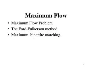
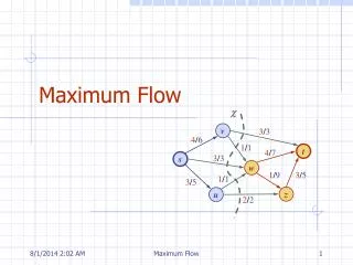
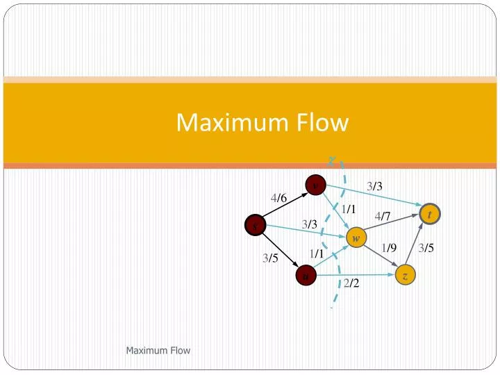
Maximum Flow. c. v. 3 / 3. 4 / 6. 1 / 1. t. 4 / 7. 3 / 3. s. w. 1 / 9. 3 / 5. 1 / 1. 3 / 5. z. u. 2 / 2. Flow Network. A flow network (or just network) N consists of

E N D
Maximum Flow c v 3/3 4/6 1/1 t 4/7 3/3 s w 1/9 3/5 1/1 3/5 z u 2/2 Maximum Flow
Flow Network • A flow network (or just network) N consists of • A weighted digraph G with nonnegative integer edge weights, where the weight of an edge e is called the capacity c(e) of e • Two distinguished vertices, s and t of G, called the source and sink, respectively, such that s has no incoming edges and t has no outgoing edges. • Example: v 3 6 1 t 7 3 s w 9 5 1 5 z u 2 Maximum Flow
Flow • A flow f for a network N is is an assignment of an integer value f(e) to each edge e that satisfies the following properties: Capacity Rule: For each edge e, 0 f (e) c(e) Conservation Rule: For each vertex v s,twhere E-(v) and E+(v) are the incoming and outgoing edges of v, resp. • The value of a flow f , denoted |f|, is the total flow from the source, which is the same as the total flow into the sink • Example: v 1/3 2/6 1/1 t 3/7 3/3 s w 2/9 4/5 1/1 3/5 z u 2/2 Maximum Flow
Maximum Flow • A flow for a network N is said to be maximum if its value is the largest of all flows for N • The maximum flow problem consists of finding a maximum flow for a given network N • Applications • Hydraulic systems • Electrical circuits • Traffic movements • Freight transportation v 1/3 2/6 1/1 t 3/7 3/3 s w 2/9 4/5 1/1 3/5 z u 2/2 Flow of value 8 = 2 + 3 + 3 = 1 + 3 + 4 v 3/3 4/6 1/1 t 3/7 3/3 s w 2/9 4/5 1/1 3/5 z u 2/2 Maximum flow of value 10 = 4 + 3 + 3 = 3 + 3 + 4 Maximum Flow
Greedy may not work • If we just keep picking paths and adding them to the flow, we may make a mistake. • In this case, sending 2 units along s-v-w-t is a mistake v 0/3 2/2 2/2 t 5/5 3/6 s w 1/1 5/5 1/1 5/5 z u 4/4 Flow of value 10 = 2 + 3 + 5 = 1 + 5 + 4 v 2/3 2/2 0/2 t 5/5 5/6 s w 1/1 5/5 1/1 5/5 z u 4/4 Maximum flow of value 12 = 2+5+5 = 2+0+5+1+4 Maximum Flow
Cut • A cut of a network N with source s and sink t is a partition c= (Vs,Vt) of the vertices of N such that sVsandtVt • Forward edge of cut c: origin in Vsand destination inVt • Backward edge of cut c: origin in Vtand destination inVs • Flow f(c) across a cut c: total flow of forward edges minus total flow of backward edges • Capacity c(c) of a cut c: total capacity of forward edges • Example: • c(c) = 24 • f(c) = 8 c v 3 6 1 t 7 3 s w 9 5 1 5 z u 2 c v 1/3 2/6 1/1 t 3/7 3/3 s w 2/9 4/5 1/1 3/5 z u 2/2 Maximum Flow
Flow and Cut Lemma: The flow f(c) across any cut c is equal to the flow value |f| Lemma: The flow f(c) across a cut c is less than or equal to the capacity c(c) of the cut Theorem: The value of any flow is less than or equal to the capacity of any cut, i.e., for any flow f and any cut c, we have|f| c(c) c1 c2 v 1/3 2/6 1/1 t 3/7 3/3 s w 2/9 4/5 1/1 3/5 z u 2/2 c(c1) = 12 = 6 + 3 + 1 + 2 c(c2) = 21 = 3 + 7 + 9 + 2 |f| = 8 Maximum Flow
Augmenting Path • Consider a flow f for a network N • Let e be an edge from u to v: • Residual capacity of e from u to v: Df(u, v) = c(e) -f (e) • Residual capacity of e from v to u: Df(v, u) = f (e) • (we can go backwards along edge) • Let p be a path from s to t • The residual capacity Df(p) ofpis the smallest of the residual capacities of the edges of p in the direction from s to t • A path p from s to t is an augmenting path if Df(p) > 0 p v 1/3 2/6 1/1 t 2/7 3/3 s w 2/9 4/5 0/1 2/5 z u 2/2 Df(s,u) = 3 Df(u,w) = 1 Df(w,v) = 1 Df(v,t) = 2 Df(p) = 1 |f| = 7 Maximum Flow
p v 1/3 2/6 1/1 t 2/7 3/3 s w 2/9 4/5 0/1 2/5 z u 2/2 p v 2/3 2/6 0/1 t 2/7 3/3 s w 2/9 4/5 1/1 3/5 z u 2/2 Flow Augmentation Lemma: Let p be an augmenting path for flow f in network N. There exists a flow f for N of value| f| = |f | +Df(p) Proof: We compute flow f by modifying the flow on the edges of p • Forward edge:f(e) = f(e) + Df(p) • Backward edge:f(e) = f(e) - Df(p) | f| = 7 Df(p) = 1 | f| = 8 Maximum Flow
Ford-Fulkerson’s Algorithm • Initially, f(e) = 0 for each edge e • Repeatedly • Search for an augmenting path p • Augment by Df(p) the flow along the edges of p • A specialization of DFS (or BFS) searches for an augmenting path • An edge e is traversed from u to v provided Df(u, v) > 0 AlgorithmFordFulkersonMaxFlow(N) for all e G.edges() setFlow(e, 0) whileGhas an augmenting path p { compute residual capacity D of p } D for all edgese p { compute residual capacity d of e } ife is a forward edge of p dgetCapacity(e) - getFlow(e) else{ e is a backward edge } dgetFlow(e) ifd<D D d { augment flow along p } for all edgese p ife is a forward edge of p setFlow(e, getFlow(e) + D) else{ e is a backward edge } setFlow(e, getFlow(e) - D) Maximum Flow
Example - Try a greedy algorithm, but be unlucky v 0/2 0/3 0/3 t 0/3 0/2 s w 0/2 0/5 0/4 0/5 z u 0/4
Example v 0/2 2/3 v 0/2 2/3 0/3 t 3/3 0/3 0/2 s t 3/3 0/2 w s 2/2 4/5 w 3/4 5/5 0/2 0/5 3/4 3/5 z u 2/4 z u 0/4 No more forward flow without pushing back v 2/2 v 0/2 2/3 0/3 0/3 t 3/3 0/3 t 2/2 3/3 s 0/2 s w w 2/2 4/5 3/4 0/2 2/5 5/5 3/4 5/5 z u 2/4 z u 2/4
Example (cont) v 2/2 v 2/2 2/3 3/3 0/3 t 3/3 2/3 t 3/3 2/2 s 2/2 s w w 2/2 4/5 3/4 2/2 5/5 5/5 2/4 5/5 z u 2/4 z u 3/4 Notice: This is clearly optimal, as the arcs into t (and leaving s) are filled. If ANY cut is maxed out, we can’t do better. Notice the effects of pushing backwards along an arc. We don’t REALLY require the flow goes forward and then backward. It is like we could change our mind while still making progress.
Analysis • In the worst case, Ford-Fulkerson’s algorithm performs |f*| flow augmentations, where f* is a maximum flow • Example • The augmenting paths found alternate between p1 and p2 • The algorithm performs 100 augmentations • Finding an augmenting path and augmenting the flow takes O(n + m) time • The running time of Ford-Fulkerson’s algorithm is O(|f*|(n + m)) v 0/50 1/50 s 1/1 t p1 1/50 0/50 u v 1/50 1/50 s 0/1 t p2 1/50 1/50 u Maximum Flow
Ford-Fulkerson Algorithm Details • Traversal can DFS or BFS, modify graph to include out-edges whose capacity is unused capacity and reversed flow edges who capacity is the flow they carry • Might only increase flow by 1 each time • O(|f*|m), pseudo-polynomial time (depends on the magnitude of a parameter not its encoding size) Maximum Flow
Edmonds-Karp Algorithm • Find the best augmenting paths, those with the fewest of edges. Greedy algorithm, like Prim’s. • Each time we choose a path, the number of edges along an augmenting path to any vertex can’t decrease. • But in turn, this implies that no edge can be a bottleneck (the smallest capacity) more than n times. • m edges can be a bottleneck n times • O(nm2) Maximum Flow
Matchings • Kindergarten Teacher needs partners for a field trip Maximum Flow
Maximum Bipartite Matching • Bipartite graphs – edges only between elements of two separate sets of vertices • Example:Jobs and Students. WorkAt edges link Students to Job. Can’t have edges from Students to Students. • Dancing, room scheduling (maximum number of classes simultaneously) • What if company has two jobs to fill? Maximum Flow
Bipartite matching In a bipartite match, all arcs go between verticies of different sets. You want to maximize the number of matches Sometimes a bipartite matching problem is modeled as a network flow problem. Can you see how? Maximum Flow
Maximum Bipartite Matching, solved by maximum flow • Direct edges, assign capacity 1 • Add source, sink, add edges to/from other nodes with capacity m. • Find maximal flow for maximal matching • Conservation => no sharing of vertices • Use regular FordFulkerson as flow is quite small. O(f*m) but our F* is <n/2 • O(nm) Maximum Flow
Maximum Bipartite Matching (transform into network flow) x: students y:jobs arc: “will work/will hire” Maximum Flow
Maximum Bipartite Matching (transform into network flow) x: students y:jobs arc: “will work/will hire” Maximum Flow
Minimum Cost flow(another version of network flow) • Add another “weight”, called cost, to edges to denote the cost to send a unit of flow along that leg. • Now, the cost of a flow is the sum of products of flow and costs on all edges • the cost of an augmenting path is the sum of forward edge costs minus the sum of backward costs • We want minimal cost for a given |f| • An augmenting cycle for a flow has same |f| (since it’s a cycle) but lower flow cost Maximum Flow
Augmenting Cycles • Given an augmenting cycle, there is a new flow whose value is the same but whose cost is augmented by w(γ)fΔ(γ) • A flow is minimum cost there is no negative-cost augmenting cycle for it Maximum Flow
Bellman-Ford Algorithm(recall from chapter 7) • A better idea is just to continually add the cheapest augmenting paths • Works even with negative-weight edges • Initially all nodes are • Must assume directed edges (for otherwise we would have negative-weight cycles) • Iteration i finds all shortest paths that use i edges. • Running time: O(nm). AlgorithmBellmanFord(G, s) for all v G.vertices() ifv= s setDistance(v, 0) else setDistance(v, ) for i 1 to n-1 do for each e =(u,z) G.edges() { relax edge e } r getDistance(u) + weight(e) ifr< getDistance(z) setDistance(z,r) Maximum Flow
Residual graph is shown on right Find cheapest path by looking at edge costs. Send maximal flow along that path Maximum Flow