Download
1 / 19
190 likes | 199 Views
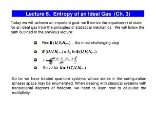
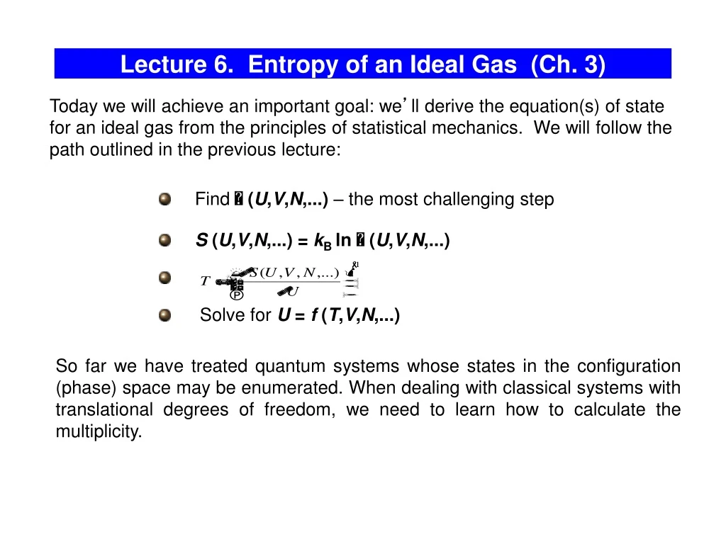
Lecture 6. Entropy of an Ideal Gas (Ch. 3). Today we will achieve an important goal: we ’ ll derive the equation(s) of state for an ideal gas from the principles of statistical mechanics. We will follow the path outlined in the previous lecture:.

E N D
Lecture 6. Entropy of an Ideal Gas (Ch. 3) Today we will achieve an important goal: we’ll derive the equation(s) of state for an ideal gas from the principles of statistical mechanics. We will follow the path outlined in the previous lecture: • Find (U,V,N,...) – the most challenging step • S (U,V,N,...)= kB ln (U,V,N,...) • Solve for U= f (T,V,N,...) So far we have treated quantum systems whose states in the configuration (phase) space may be enumerated. When dealing with classical systems with translational degrees of freedom, we need to learn how to calculate the multiplicity.
Multiplicity for a Single particle • depends on three rather than two macro parameters (e.g., N, U, V). Example: particle in a one-dimensional “box” -L L The total number of ways of filling up the cells in phase space is the product of the number of ways the “space” cells can be filled times the number of ways the “momentum” cells can be filled px Quantum mechanics (the uncertainty principle) helps us to numerate all different states in the configuration (phase) space: -L L x px -px x Q.M. The number of microstates:
n p Multiplicity of a Monatomic Ideal Gas (simplified) For a molecule in a three-dimensional box: the state of the molecule is a point in the 6D space - its position (x,y,z) and its momentum (px,py,pz). The number of “space” microstates is: For N molecules: There is some momentum distribution of molecules in an ideal gas (Maxwell), with a long “tail” that goes all the way up to p = (2mU)1/2 (U is the total energy of the gas). However, the momentum vector of an “average” molecule is confined within a sphere of radius p ~ (2mU/N)1/2 (U/N is the average energy per molecule). Thus, for a single “average” molecule: The total number of microstates for N molecules: However, we have over-counted the multiplicity, because we have assumed that the atoms are distinguishable. For indistinguishable quantum particles, the result should be divided by N! (the number of ways of arranging N identical atoms in a given set of “boxes”):
pz py px More Accurate Calculation of N (I) Momentum constraints: 1 particle - 2 particles - The accessible momentum volume for N particles = the “area” of a 3N-dimensional hyper-sphere p N =1 The reason why m matters: for a given U, a molecule with a larger mass has a larger momentum, thus a larger “volume” accessible in the momentum space. Monatomic ideal gas: (3N degrees of freedom) f N- the total # of “quadratic” degrees of freedom
pz py px More Accurate Calculation of N (II) For a particle in a box (L)3: (Appendix A) If p>>p, the total degeneracy (multiplicity) of 1 particle with energy U is: If p>>p, the total degeneracy (multiplicity) of N indistinguishable particle with energy U is: Plug in the “area” of the hyper-sphere:
Entropy of an Ideal Gas The Sackur-Tetrode equation: (Monatomic ideal gas) an average volume per molecule an average energy per molecule In general, for a gas of polyatomic molecules: f 3 (monatomic), 5 (diatomic), 6 (polyatomic)
Two cylinders (V = 1 liter each) are connected by a valve. In one of the cylinders – Hydrogen (H2) at P = 105 Pa, T = 200C , in another one – Helium (He) at P = 3·105 Pa, T=1000C. Find the entropy change after mixing and equilibrating. Problem For each gas: The temperature after mixing: H2 : He:
Consider two different ideal gases (N1, N2) kept in two separate volumes (V1,V2) at the same temperature. To calculate the increase of entropy in the mixing process, we can treat each gas as a separate system. In the mixing process, U/N remains the same (T will be the same after mixing). The parameter that changes is V/N: Entropy of Mixing if N1=N2=1/2N , V1=V2=1/2V The total entropy of the system is greater after mixing – thus, mixing is irreversible.
Gibbs “Paradox” - applies only if two gases are different ! If two mixing gases are of the same kind (indistinguishable molecules): Stotal = 0 because U/N and V/N available for each molecule remain the same after mixing. Quantum-mechanical indistinguishability is important! (even though this equation applies only in the low density limit, which is “classical” in the sense that the distinction between fermions and bosons disappear.
Problem Two identical perfect gases with the same pressure P and the same number of particles N, but with different temperatures T1 and T2, are confined in two vessels, of volume V1 and V2 , which are then connected. find the change in entropy after the system has reached equilibrium. - prove it! at T1=T2, S=0, as it should be (Gibbs paradox)
An Ideal Gas: from S(N,V,U) - to U(N,V,T) Ideal gas: (fN degrees of freedom) - the “energy” equation of state - in agreement with the equipartition theorem, the total energy should be ½kBT times the number of degrees of freedom. The heat capacity for a monatomic ideal gas:
Partial Derivatives of the Entropy We have been considering the entropy changes in the processes where two interacting systems exchanged the thermal energy but the volume and the number of particles in these systems were fixed. In general, however, we need more than just one parameter to specify a macrostate, e.g. for an ideal gas When all macroscopic quantities S,V,N,U are allowed to vary: We are familiar with the physical meaning only one partial derivative of entropy: Today we will explore what happens if we let the V vary, and analyze the physical meaning of the other two partial derivatives of the entropy:
Mechanical Equilibrium and Pressure UA, VA, NA UB, VB, NB S AB S A S B VA VAeq Let’s fix UA,NA and UB,NB , but allow V to vary (the membrane is insulating, impermeable for gas molecules, but its position is not fixed). Following the same logic, spontaneous “exchange of volume” between sub-systems will drive the system towards mechanical equilibrium (the membrane at rest). The equilibrium macropartition should have the largest (by far) multiplicity (U, V) and entropy S (U, V). In mechanical equilibrium: e.g. ideal gas - the volume-per-molecule should be the same for both sub-systems, or, if T is the same, P must be the same on both sides of the membrane. The stat. phys. definition of pressure:
The “Pressure” Equation of State for an Ideal Gas The “energy” equation of state (U T): Ideal gas: (fN degrees of freedom) The “pressure” equation of state (P T): - we have finally derived the equation of state of an ideal gas from first principles!
i.e. Thermodynamic identity I Let’s assume N is fixed, thermal equilibrium: mechanical equilibrium:
Quasi-Static Processes (all processes) (quasi-static processes with fixed N) Thus, for quasi-static processes : Comment on State Functions : P - is an exact differential (S is a state function). Thus, the factor 1/T converts Q into an exact differential for quasi-static processes. V Quasistatic adiabatic (Q = 0) processes: isentropic processes The quasi-static adiabatic process with an ideal gas : - we’ve derived these equations from the 1st Law and PV=RT On the other hand, from the Sackur-Tetrode equation for an isentropic process :
(all the processes are quasi-static) Problem: (a) Calculate the entropy increase of an ideal gas in an isothermal process. (b) Calculate the entropy increase of an ideal gas in an isochoric process. You should be able to do this using (a) Sackur-Tetrode eq. and (b) Let’s verify that we get the same result with approaches a) and b) (e.g., for T=const): Since U = 0, (Pr. 2.34)
Problem: • A bacterias of mass M with heat capacity (per unit mass) C, initially at temperature T0+T, is brought into thermal contact with a heat bath at temperatureT0.. • (a) Show that if T<<T0, the increase S in the entropy of the entire system (body+heat bath) when equilibrium is reached is proportional to (T)2. • Find S if the body is a bacteria of mass 10-15kg with C=4 kJ/(kg·K), T0=300K, T=0.03K. • What is the probability of finding the bacteria at its initial T0+T for t =10-12s over the lifetime of the Universe (~1018s). (a) (b)
Problem (cont.) for the (non-equilibrium) state with Tbacteria = 300.03K is greater than in the equilibrium state with Tbacteria = 300K by a factor of (b) The number of “1ps” trials over the lifetime of the Universe: Thus, the probability of the event happening in 1030 trials: