Download
1 / 32
320 likes | 424 Views
Seasonal Prediction with CCSM3.0: Impact of Atmosphere and Land Surface Initialization.

E N D
Seasonal Prediction with CCSM3.0: Impact of Atmosphere and Land Surface Initialization Jim Kinter1Dan PaolinoDavid Straus1Ben Kirtman2Dughong Min2Center for Ocean-Land-Atmosphere Studies1 also George Mason University thanks to NCAR CISL for2 University of Miami computing resources
Climate Sensitivity to Land Surface Conditions Wet Soil Dry Soil July Precipitation July Temperature Shukla and Mintz, 1982 Influence of Land-Surface Evapotranspiration on the Earth's Climate. Science, 215, 1498-1501.
Global Land-AtmosphereCoupling Experiment GLACE showed that coupling between land and atmosphere is strongest in transitional zones between humid and arid regions (and lots of inter-model variance!). Koster et al., 2004 Koster, R. D., P. A. Dirmeyer, Z. Guo, G. Bonan, E. Chan, P. Cox, H. Davies, T. Gordon, S. Kanae, E. Kowalczyk, D. Lawrence, P. Liu, S. Lu, S. Malyshev, B. McAvaney, K. Mitchell, T. Oki, K. Oleson, A. Pitman, Y. Sud, C. Taylor, D. Verseghy, R. Vasic, Y. Xue, and T. Yamada, 2004: Regions of strong coupling between soil moisture and precipitation. Science, 305, 1138-1140.
Land-Atmosphere Interactions over the Great Plains • Coupling strength from Koster, Dirmeyer, Guo et al. (2004) showing “hotspots” for land-atmosphere coupling • Estimate of “GLACE diagnostic”* from 12 land surface models (Guo et al. 2007) • COLA GCM (10-year integration with specified observed SST) anomaly correlation of Ts (horizontal scale) and change in correlation when observed vegetation properties are specified (vertical scale; Gao et al. 2007) * Evaporation variability times a land-atmospheric flux function based on the tightness of the dependence of surface fluxes on soil moisture
Soil Moisture Memory Enhances Predictability GSWP-2 results from multiple models provide quantitative information about the effect of soil moisture on predictability. The season (color) and duration (intensity) of the maximum soil moisture memory is shown. Series of papers by Guo and Dirmeyer; Guo et al.; Seneviratne et al.
GLACE2 - Forecast Correlation Precipitation Temperature Evaporation Soil Moisture 100 initial times: 10 years (1986-1995) X 5 months (Apr.-Aug.) X 2 days (the 1st and 15th) 10-member, 2-month COLA AGCM runs with observed SST Correlations for CONUS region average: 70-125W, 22-50N ______ realistic land ICs runs ______ random land ICs runs ---------- 95% significance level Courtesy of Zhichang Guo
Model: CCSM3.0 is a coupled ice-ocean-atmosphere-land climate model with state-of-the-art formulations of dynamics and subgrid-scale physical parameterizations. The atmosphere is CAM3 (Eulerian dynamical core) at T85 (~150 km) horizontal resolution with 26 vertical levels. The ocean is POP with 1 degree resolution, stretched to 1/3 degree near the equator. Re-forecast Experiments: Retrospective forecasts cover the period 1982–1998 for the July initial state experiments, and 1981-2000 for the January initial state experiments. Ensembles of 6 (10) hindcasts were run in the OCN-only (ATM-OCN-LND) experiments (see below). Ocean Initialization: The ocean initialization uses the GFDL ocean data assimilation system, based on the MOM3 global ocean model using a variational optimal interpolation scheme. The GFDL ocean initial states were interpolated (horizontally and vertically) to the POP grid using a bi-linear interpolation scheme. (Climatological data from long simulations of CCSM3 were used poleward of 65°N and 75°S.) The ocean initial state is identical for each ensemble member. EXPERIMENTSOne-year re-forecast ensembles with CCSM3.0 Initial states: 1 January and 1 July for 1981-2000Two sets of re-forecasts
Land/Atmosphere Initial Conditions in Two Sets of Experiments OCN-only Experiment The atmospheric and land surface initial states were taken from an extended atmosphere/land-only (CAM3) simulation with observed, prescribed SST. The atmospheric ensemble members were obtained by resetting the model calendar back one week and integrating the model forward one week with prescribed observed SST. In this way, it is possible to generate initial conditions that are synoptically independent (separated by one week) but have the same initial date. Thus all ensemble members were initialized at the same model clock time (1 Jan or 1 July) with independent atmospheric initial conditions.
Land/Atmosphere Initial Conditions in Two Sets of ExperimentsATM-OCN-LND ExperimentLand and atmosphere were initialized for each of the 10 days preceding the date of each ocean initial state * 22-31 December for the 1 January ocean states * 22-30 June for the 1 July ocean datesAtmosphere initialized by interpolating from daily Reanalysis. Land surface initialized from daily GSWP (1986-1995) and daily ERA40 (1982-1985 and 1996-1998). Observed anomalies superimposed on Common Land Model (CLM) climatology. Snow cover initialized from ERA40. Sea-ice initialized to climatological monthly condition based on a long simulation of CCSM3.0.
CCSM Performance - Predicting ENSO CFS CCSM OISST Jan 1983 Jan 1988 Time-longitude cross-sections of equatorial Pacific SST anomaly
CCSM Re-Forecast Examples - Jul 1984 ERA-40 1-month lead 1-month lead ATM-OCN-LND OCN CFS 7-month lead 7-month lead 7-month lead
CCSM Re-Forecast Examples - Jul 1984 ERA-40 1-month lead 1-month lead ATM-OCN-LND OCN CFS 7-month lead 7-month lead 7-month lead
CCSM Re-Forecast Examples - Jul 1984 ERA-40 1-month lead 1-month lead ATM-OCN-LND OCN CFS 7-month lead 7-month lead 7-month lead
CCSM Re-Forecast Examples - Jul 1986 ERA-40 1-month lead 1-month lead ATM-OCN-LND OCN CFS 7-month lead 7-month lead 7-month lead
CCSM Re-Forecast Examples - Jul 1986 ERA-40 1-month lead 1-month lead ATM-OCN-LND OCN CFS 7-month lead 7-month lead 7-month lead
CCSM Re-Forecast Examples - Jul 1986 ERA-40 1-month lead 1-month lead ATM-OCN-LND OCN CFS 7-month lead 7-month lead 7-month lead
CCSM Re-Forecast Examples - Jul 1989 ERA-40 1-month lead 1-month lead ATM-OCN-LND OCN CFS 7-month lead 7-month lead 7-month lead
CCSM Re-Forecast Examples - Jul 1989 ERA-40 1-month lead 1-month lead ATM-OCN-LND OCN CFS 7-month lead 7-month lead 7-month lead
CCSM Re-Forecast Examples - Jul 1989 ERA-40 1-month lead 1-month lead ATM-OCN-LND OCN CFS 7-month lead 7-month lead 7-month lead
CCSM Re-Forecast Examples - Jul 1992 ERA-40 1-month lead 1-month lead ATM-OCN-LND OCN CFS 7-month lead 7-month lead 7-month lead
CCSM Re-Forecast Examples - Jul 1992 ERA-40 1-month lead 1-month lead ATM-OCN-LND OCN CFS 7-month lead 7-month lead 7-month lead
CCSM Re-Forecast Examples - Jul 1992 ERA-40 1-month lead 1-month lead ATM-OCN-LND OCN CFS 7-month lead 7-month lead 7-month lead
(Top) Soil Moisture Prediction Skill CCSM top 9 cm ERA40 top 7 cm ATM-OCN-LND CCSM top 9 cm ERA40 top 7 cm OCN July (1-month lead) Soil Moisture (top level) Prediction Skill
(Mid) Soil Moisture Prediction Skill CCSM 9-29 cm ERA40 7-28 cm ATM-OCN-LND CCSM 9-29 cm ERA40 7-28 cm OCN July (1-month lead) Soil Moisture (mid-level) Prediction Skill
Model Drydown 7-month lead (Jan ICs) vs. 1-month lead (Jul ICs) - percent difference ATM-OCN-LND OCN-only CFS
Global Surface Air Temperature Forecasts JAN: 1-month lead FEB: 2-month lead Simultaneous correlation CCSM forecasts CAMS analysis January initial conditions ATM-OCN-LND ATM-OCN-LND OCN OCN
Global Precipitation Forecasts for July Simultaneous correlation for July initial conditions, 1-month lead forecasts and CMAP ATM-OCN-LND OCN
Indian Monsoon Rainfall The JAS mean precipitation in south Asia. ATM-OCN-LND OCN The simulated interannual variability of JAS rain over land (not shown) is much smaller than observed. CMAP
Nordeste Brazil Forecast 1 January ICs ATM-OCN-LND OCN-only CMAP
Interannual Variability of Indian Monsoon Circulation Leading EOF of JAS mean 850 hPa rotational winds, 1982-1998. ERA40ATM-OCN-LNDOCN-only
Summary • Sensitivity of seasonal climate to land surface conditions is well-established • Varies with phase of annual cycle • Varies with climate regime: highest sensitivity in semi-arid regions • Clear improvement of sub-seasonal regional surface climate anomalies associated with initializing land surface • At seasonal time scales, situation is more mixed • SST forecast plays first-order role, i.e., places where SST is major determinant of seasonal climate have little sensitivity to land surface initialization, and initializing land surface cannot compensate for bad SST forecast • Improvements in seasonal forecast skill due to initializing land surface are modest • Improvements in cold season associated with snow initialization • Land surface bias that evolves with forecast lead time remain a big problem