Download
1 / 79
790 likes | 815 Views
Acceleration of Cosmic Rays. Pankaj Jain IIT Kanpur. spectrum. Flux: number ------------------- m 2 sr s GeV. Knee at 10 15 eV The spectrum steepens after the knee, Ankle at 10 18.5 eV ,

E N D
Acceleration of Cosmic Rays Pankaj Jain IIT Kanpur
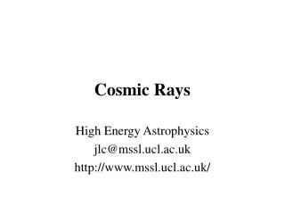
spectrum Flux: number ------------------- m2 sr s GeV Knee at 1015 eV The spectrum steepens after the knee, Ankle at 1018.5 eV, perhaps an indication of a change over from galactic to extragalactic origin
Spectrum KNEE ANKLE
Spectral Index • Flux 1/E • = 2.7 1015 eV<E<109 eV • = 3.1 1018.5 eV>E >1015 eV • 2.7 E>1018.5 eV At higher energies spectrum again becomes steeper ( > 4)
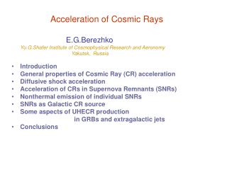
Origin • The high energy cosmic rays probably arise due to acceleration of charged particles at some astrophysical sites • supernova shock waves • Active galactic nuclei • gamma ray bursts • pulsars • galaxy mergers Bottom up model
Origin Alternatively very massive objects might decay in our galaxy and produce the entire spectrum of high energy cosmic rays The massive objects would be a relic from early universe with mass M > 1015 mass of proton Top Down Model
Origin These massive objects could be: Topological defects Super heavy particles Primordial black holes
Origin Here we shall focus on the Bottom Up Model where the particles are accelerated at some astrophysical sites
Our astrophysical neighbourhood Distance to nearest star 1.3 pc (4 light years) Milky way disk diameter 30 Kpc Galaxies also arrange themselves in Groups or clusters These further organize in super clusters, size about 100 Mpc Beyond this universe is isotropic and homogeneous
Distribution of galaxies in our neighbourhood CFA Survey 1986
2dF Galaxy Redshift Survey 3D location of 230 000 galaxies
As we go to distances larger than 100 Mpc we enter the regime of cosmology z = v/c = H0 d (Hubble Law) z 1 at distances of order 1 Gpc As we go to large z (or distance), the Universe looks very different. It has much higher population of exotic objects like Active Galactic Nuclei Gamma Ray Bursts
Acceleration Mechanisms Fermi acceleration Betatron acceleration: acceleration due to time varying electromagnetic fields
Fermi Acceleration: Basic Idea Charged particles are accelerated by repeatedly scattering from some astrophysical structures Ex: Supernova shock waves, magnetic field irregularities At each scattering particles gain a small amount of energy Particles are confined to the acceleration site by magnetic field Shock wave
Supernova Explosion Stars more massive than 3 solar masses end their life in a supernova explosion. This happens when either C or O is ignited in the core. The ignition is explosive and blows up the entire star. For more massive stars the core becomes dominated by iron. Explosion occurs due to collapse of the iron core. The core becomes a neutron star or a black hole
Supernova Explosion Supernova explosions also happen in binary star systems In this case one of the stars accretes or captures matter from its binary partner, becomes unstable and explodes For example, the star may be a white dwarf MWD < 1.44 Solar Mass Chandrasekhar limit If its mass exceeds this limit, it collapses and explodes into a supernova
Supernova Explosion 0.1 sec 0.5 sec 2 hours Brightens by 100 million times months
Supernova Explosion, Aftermath The explosion sends out matter into interstellar space at very high speed, exceeding the sound speed in the medium, leading to a strong shock wave For sufficiently massive star the core becomes a pulsar (neutron star) or a black hole
Brightest supernova observed SN1006 visible in day time 3 times size of Venus Intensity comparable to Moon
Remnant of the Supernova explosion seen in China in AD1054 (Crab Nebula) also observable in day time Expansion: angular size increasing at rate 1.6’’ per 10 years
Magnetic Fields in Astrophysics Magnetic fields are associated with almost all astrophysical sites Our galaxy has a magnetic field of mean strength 3 G The field is turbulent
Magnetic Fields in Astrophysics Cosmic rays are confined at the astrophysical sites by magnetic field They may also scatter on the magnetic field irregularities and gain or loose energy
particles may gain energy by scattering on astrophysical structures U Magnetic cloud
y S: observer x Fermi Acceleration: simple example Mass U
y’ S’ x’ y S: observer x Fermi Acceleration: simple example In S’: vi’ = v vf’ = -v v Elastic scattering -v U In S: vi = v – U vf = - v – U= - vi - 2U net gain in speed
simple example cont’ Gain in energy per scattering: E = Ef – Ei = (1/2) m (v+U)2 – (1/2) m (v-U)2 = 2mvU = 2mvi U + 2m U2
particles move at speed close to the speed of light. Hence we need to make a relativistic calculation at oblique angles v c (velocity of light) U << c
y S: observer x Relativistic calculation Frame S: angle of incidence = Ei = E Pi = P U
y’ S’ x’ Relativistic calculation Frame S’: pix’ = (Px + E U/c2) Ei’ = (E + UPx) Pfx’ = - Pix’ Ef’ = Ei’ Pix’ “Mirror” -Pix’ U Frame S: Ef = (Ef’ – UPfx’)
Relativistic calculation cont’ Gain in energy per scattering: Particles will gain or loose energy depending on the angle of incidence
Fermi Acceleration Lets assume that initially N0 charged particles with mean energy E0 per particle are confined in the accelerating region by magnetic field. they undergo repeated interactions with the magnetic clouds
Fermi Acceleration Charged particles are accelerated by repeatedly scattering from some astrophysical structures per collision U = speed of structure v = speed of particle We need average E/E over many collisions
Fermi Acceleration Prob of collision v + U cos v Head on collisions are more probable U
Lets assume that initially N0 charged particles with mean energy E0 per particle are confined in the accelerating region by magnetic field After one collision E = E0 =1+(8/3) (U/c)2 Let P = probability the particle remains in the site after one collision, depends on the time of escape from the site After k collisions we have N = N0Pk particles with energy E E0 k N( E) = const Eln P/ln dN = N(E) dE = const Eln P/ln 1
N(E) dE = const Eln P/ln 1 E We have obtained a power law, as desired However it depends on details of the accelerating site such as P, . We see the same in all directions Also the mean energy gain per collision U2 Second order Fermi acceleration The process is very slow The particle might escape before achieving required energy or energy losses might become very significant
It would be nice to have a process where the particles gain energy in each encounter. In this case Achieved by Fermi First order mechanism
Reference: High Energy Astrophysics by Malcolm S. Longair
First order Fermi acceleration Particles accelerated by strong shocks generated By supernova explosion strong shock: shock speed >> upstream sound speed (104 Km/s) (10 Km/s) upstream downstream shock US assume that a flux of high energy particles exist both upstream and downstream
First order Fermi acceleration Shock front downstream V2, 2 upstream V1, 1 In shock frame US V2=|US|/4 V1=|US| 1V1 = 2V2 2/1=(+1)/( 1) = 4 for strong shocks = 5/3 monoatomic or fully ionized gas V2 = V1/4
3|US|/4 3|US|/4 isotropic isotropic First order Fermi acceleration upstream frame downstream frame The particle velocities are isotropic both upstream and downstream in their local frames. High energy particles are repeatedly brought to the shock front where they undergo acceleration at each crossing
3|US|/4 isotropic First order Fermi acceleration Consider high energy particles crossing the shock from upstream to downstream The particles hardly notice the shock Downstream medium approaches the particles at speed U = 3US/4
First order Fermi acceleration The particles undergo repeated scattering on magnetic irregularities and become isotropic in downstream medium Let’s determine the energy of the particle in the frame in which the downstream particles are isotropic
U =3US/4 upstream frame E, Px vc downstream upstream In downstream frame: E’ = (E + PxU) U<< c, 1 Velocity of particle v c E = Pc Px = (E/c) cos E’ = E + (E/c) U cos
We next average this over from 0 to /2 Rate at which particles approach the shock cos Number of particles at angle sin d =d cos Prob. of particle to arrive at shock at angle P() d = 2 cos dcos
Now the important point is that the situation is exactly identical for a particle crossing the shock from downstream to upstream 3|US|/4 downstream upstream
First order Fermi acceleration For each crossing: U = 3US/4 For each round trip = E/E0 = 1+ 4U/3c