Download
1 / 19
190 likes | 325 Views
A simple smoothed seismicity forecast for prospective testing in Japan. Jeremy Douglas Zechar Lamont-Doherty Earth Observatory. Smoothed seismicity. Physical intuition : Earthquakes do not occur at a point, they affect some (unknown) region around the hypocenter/rupture surface.

E N D
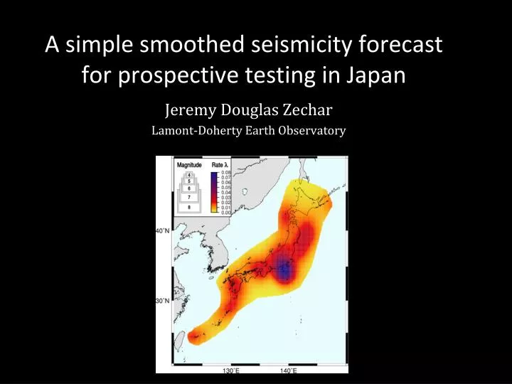
A simple smoothed seismicity forecast for prospective testing in Japan Jeremy Douglas Zechar Lamont-Doherty Earth Observatory
Smoothed seismicity • Physical intuition: Earthquakes do not occur at a point, they affect some (unknown) region around the hypocenter/rupture surface. • Mathematical representation: Therefore, each event should be smoothed somehow to represent its influence. • Resulting model: The smoothed seismicity map can serve as a reference model against which to compare more complex models.
Decisions to make • Functional form of smoothing kernel • Shape (power law, Gaussian, Epanechnikov, anistropic) • Smoothing lengthscale • Magnitude dependence • Time dependence • Declustering • Declustering itself is a modeling challenge. • Results may be unstable w/r/t parameter choices.
US National Seismic Hazard Map smoothing Binned epicenters are smoothed using Gaussian with uniform correlation distance of 50 km, following Frankel, 1995. Petersen et al.,2008
New Zealand NSHM smoothing Binned epicenters are smoothed using Gaussian with variable lengthscale, dependent on epicentral density, following Stock & Smith (2002).
Kagan& Jackson smoothing Epicenters are smoothed using a doubly truncated anisotropic power law with directionality based on focal mechanism, following Kagan and Jackson, 1994. Each epicenter’s contribution is also weighted by magnitude and time.
Helmstetter, Kagan, & Jackson smoothing • Extension of Kagan & Jackson method, using smaller events (M>=2 in CA) and an adaptive smoothing lengthscale (Helmstetteret al. 2007)
Zechar Simple Smoothed Seismicity (Triple S) • Gaussian kernel, fixed bandwidth, isotropic, time-invariant, magnitude-invariant • Bandwidth optimized using retrospective experiment • Applied globally, currently under prospective test
Hit Miss False alarm Correct negative Alarm Negative alarm Binary prediction, binary outcome Space Time
Molchan diagram Molchan, 1991, Molchan & Kagan, 1992
Generalize alarm set to alarm function Alarm function value latitude latitude longitude longitude
Molchan diagram Molchan trajectory: collection of (t,n) points generated from alarm function Potential for ambiguity
Area skill score • Area above a Molchan trajectory, cumulative measure of performance for a given alarm function f(x): • Reference model p(x) is used to define measure of space in computing t. • Typically, reference model is based on historical distribution of seismicity. • In the case when p(x) is very good, af(1) ½ for all f(x). ~ ~ Zechar & Jordan, 2008
Emphasis on reference model • One can pose the problem of earthquake prediction as the search for the distribution of seismicity, p(x). • To measure the utility of a given earthquake prediction, one can compare the predicted distribution with the observed distribution, relative to a reference model, p(x). • Understanding of earthquake predictability can progress through iterative improvement of the reference model. ~
Optimization experiment • Consider a very simple class of forecasts: • Smoothed seismicity, single lengthscale parameter • Gaussian kernel, lengthscales • We smooth a set of eqks in a learning period to forecast target eqks in the test period. • Vary the value of s. • Determine the optimal value of s for this learning period. • Goal: to construct an optimized reference model for prospective experiments
Optimal value of s • Each value of s corresponds to a unique alarm function, a candidate reference model. • The best reference model is the one which brings all others closest to af(1) = ½. This is measured by minimizing the average misfit:
Predictability experiment • Consider S = {5,10,20,25,30,50,75,100,200} km • Target earthquakes: MJMA ≥ 3.95 • Study region: Japan • Smooth MJMA ≥ 1.95 eqks, 1 Jan 2000 to 31 Dec 2003 • Test period: 1 Jan 2004 to 31 Dec 2007
Optimization results • (km) c ============== • 5 0.320 • 10 0.306 • 20 0.261 • 25 0.236 • 30 0.220 • 50 0.180 • 75 0.155 • 100 0.165 • 200 0.194
Resultant prospective forecast Testing began 1 Sep 2008 and will continue for 1 yr. Simple Smoothed Seismicity (Triple S) model is also under test in California, Western Pacific and Global testing regions.