Download
1 / 22
220 likes | 431 Views
Granulated Activated Carbon Filter Model & Simulations. Razvan Carbunescu Sarah Johnston Mona Crump Brett McCullough Daniel Guidry. What is GAC?. GAC stands for Granular Activated Carbon It is a low volume, high surface area material

E N D
Granulated Activated Carbon Filter Model & Simulations RazvanCarbunescu Sarah Johnston Mona Crump Brett McCullough Daniel Guidry
What is GAC? • GAC stands for Granular Activated Carbon • It is a low volume, high surface area material • The carbon based material is converted to activated carbon by thermal decomposition in a furnace using a controlled atmosphere and heat.
GAC Filter Description • The Glass beads and wool evenly disperse air flow. • A syringe pump empties pollutants into the air supply.
GAC Properties – Adsorption • The pores in activated carbon result in a large surface area. • A gram of activated carbon can have a surface area of 500 to 1500 meters squared. • One pound of GAC, about a quart in volume, can have a total surface area of 125 acres
Biofilter Considerations • Biofilters are sensitive to Input loading. • Too much or too little load can disrupt the effectiveness of the biofilter. • GAC filters can help to alleviate drastic oscillations in biofilter input loading by providing a steady load.
Providing a Steady State Inputto the Biofilter For Example: 500ppm typical median factory output 0ppm (no load) factory output GAC passes load through at same level GAC releases stored contaminant 500ppm GAC output / Biofilter input 500ppm GAC output / Biofilter input 1000ppm “shock loading” factory output GAC reduces excess load to biofilter 500ppm GAC output / Biofilter input
Equations – Non-linear equation 1.3 The non-linear coupling equation
Matrix Approximations We use MATLAB to calculate the matrices needed to approximate the functions More Legendre roots means a better approximation for the derivatives and a better approximation for the general functions Legendre Roots are given from the tables by Stroud and Secrest(1966) up to thirty significant digits
Matrix Approximations Radial – symmetric, spherical geometry Used to approximate the carbon beads themselves W= ( 0.09491 0.19081 0.04762 ) ( ) -15.66996 20.03488 -4.36492 9.96512 -44.33004 34.36492 26.93285 -86.9329 60.00000 B = W = ( 0.0098 0.0349 0.0635 0.0819 0.0796 0.0541 0.0095 ) ( ) -62.623 80.052 -25.737 13.188 -7.9903 4.9756 -1.8647 22.579 -82.222 75.799 -23.892 12.242 -7.1015 2.5966 -3.984 41.6 -109.32 90.627 -27.8 13.572 -4.6954 1.5827 -10.166 70.264 -166.99 132.72 -39.386 11.975 -0.98636 5.3578 -22.169 136.52 -322.49 255.95 -52.178 0.90471 -4.578 15.942 -59.671 377.01 -1024.3 694.74 46.257 -195.81 488.51 -1024.6 2044.8 -3127.2 1768 B =
Matrix Approximations Axial – non-symmetric, planar geometry Used to approximate the flow itself -3 4 -1 -1 0 1 1 -4 3 ( ) A = -43.0014 47.9927 -6.6848 2.6155 -1.6079 1.3628 -1.6765 0.9997 -18.2773 14.2907 5.1519 -1.7720 1.0498 -0.8770 1.0728 -0.6389 5.2138 -10.5516 2.3498 4.1637 -1.9552 1.5125 -1.7966 1.0636 -2.6370 4.6889 -5.3795 0.5063 4.1903 -2.5266 2.7791 -1.6215 1.6212 -2.7784 2.5267 -4.1912 -0.5051 5.3799 -4.6911 2.6381 -1.0631 1.7956 -1.5120 1.9549 -4.1617 -2.3548 10.5570 -5.2158 0.6385 -1.0720 0.8766 -1.0495 1.7711 -5.1525 -14.2884 18.2761 -0.9997 1.6765 -1.3628 1.6079 -2.6155 6.6848 -47.9927 43.0014 ( ) A =
Legendre Roots Axial roots for non-symetric planar geometry now calculated Radial roots not necessary for calculations Matlab program solves for the roots of the equations after polynomial is formed Limited to 80 roots for non-symmetric and 40 roots for symmetric because of the size of the polynomial coeficients
New GAC Filter Interface Based on the old interface combined with the matlab program Integrates the resulting graph into the interfcace Allows for modification of the discretization accuracy Has initial parameters set
New GAC Filter Interface (cont) Allows for the specification if the input concentration from an external excel file Allows for specification of the type of input concentration (steady, intermitent, …) Allows for the results of the simulation to be saved to an excel file for later use Allows for adding an experimental data set to the graph to compare results
3 Axial Points 3 Radial Points • Comparison of experimental results versus simulation results with 3 axial points and 3 radial points
5 Axial Points 3 Radial Points • Comparison of experimental results versus simulation results with 5 axial points and 3 radial points
7 Axial Points 3 Radial Points • Comparison of experimental results versus simulation results with 7 axial points and 3 radial points