Download
1 / 27
280 likes | 446 Views
Big Data. Fast Data. June 2011. Ryan Betts, VoltDB Engineering. rbetts@voltdb.com / @ ryanbetts. Volume. Velocity. Variation. http://jtonedm.com/2011/05/24/ibms-big-data-platform-and-decision-management / Analyzing streaming data to find patterns

E N D
Big Data. Fast Data. June 2011 Ryan Betts, VoltDB Engineering rbetts@voltdb.com / @ryanbetts
Volume. Velocity. Variation. http://jtonedm.com/2011/05/24/ibms-big-data-platform-and-decision-management/ • Analyzing streaming data to find patterns • Analyzing streaming data to make decisions. James Taylor on Everything Decision Management
The Problem Throughput: Lots of transactions: 10,000 to 1M TPS Cost: Cheap transactions: $ / transaction must be tiny Scale: Streaming writes. Reads of summary aggregates
Giant score board in the sky Financial tick streams 100k to 2M write/update TPS 1000’s of summary read TPS Sensor inputs 50k – 500k writes/update TPS 100’s summary read TPS
Transaction Mix Lower-frequency transactions High-frequency transactions DataSource Financial trademonitoring Digital Advertising Telco call data record management Website vulnerability detection Online gaming micro transactions Package tracking(logistics)
Big Data Challenges Big Data and You You need to validatein real-time You need to countand aggregate You need to enrichin real-time You need to scale on demand You need to learnand adapt
VoltDB and big data Throughput: Design choices favor throughput. Cost: Commodity hardware. Efficient. Open source. Scale: Clustered. Shared nothing. Clever. Originated from MIT / Brown / Yale H-Store research project. http://cs-www.cs.yale.edu/homes/dna/papers/vldb07hstore.pdf
Decision: Scale horizontally Replicate for fault tolerance
Decision: Transaction == Stored Procedure SQL for data access Java for user procedure logic
Decision: Eliminate stalls during transactions No disk waits during a transaction No server <-> client network chatter
Decision: Concurrency by scheduling not by locking
Decision: ACID / Transactional CAP-wise consistent
Decisions lead to: ACID & Throughput Per node: • 1 million SQL statements per second • 50,000 multi-statement procedures per second Per node TPC-C TPS on 3 and 6 nodes:
How: Data Tables are horizontally split into PARTITIONS
How: Processing Procedures routed to, ordered and run at partitions
VoltDB procedures Transaction == stored procedure invocation. Two procedure types – both ACID Single-Partition All SQL operates within a single partition Multi-Partition SQL operations on partitioned tables across partitions Insert/update/delete on replicated data
Running transactions • Single-threaded executor at each partition • No locking/dead-locks • Transactions run to completion, serially, at each partition • Single partition procedures run in microseconds • However, single-threaded comes at a price • Other transactions wait for running transaction to complete • Don’t do anything crazy in a procedure (request web page, send email)
A stored procedure @ProcInfo(singlePartition=true, partitionInfo=“tags.tag: 0”) public class Insert extendsVoltProcedure { public final SQLStmtsql = newSQLSmt( “INSERT INTO hashtags (tag, tweet_ts) VALUES (?,?);”); publicVoltTable[] run(String tag, long timestamp) throws… { voltQueueSQL(sql, tag, timestamp); returnvoltExecuteSQL(true); } }
X X X X X Physical schema • Tables Partitioned Rows spread across cluster by table column High frequency of modification (transactional data) Replicated All rows exists in all VoltDB partitions Low frequency of modification (customers, city, state, …) Materialized Views Grouped, aggregated partitioned table data Automatically updated as table data is changed Export-only tables Insert-only tables Produces an externally consumable data stream • Indexes – composite keys, unique, non-unique
Example View -- Agg. votes by contestant. Determine winner create view votes_by_contestant( contestent_number, num_votes) as select contestant_number, count(*) fromvotes group by contestant_number;
VoltDB Applications Develop: Schema and procedures Assemble: using VoltCompiler to prepare procedures Deploy: application JAR file Monitor: log4j, built-in stats procedures, memory monitor, VoltDB Enterprise Manager (commercial)
Client Applications Client application decisions Language: Java, C#, C++, PHP, Python, Ruby, Erlang Protocol: Wire or HTTP/JSON If wire then Asynchronous or Synchronous General client application structure Connect to one or more nodes Transactions are forwarded to appropriate node in the cluster Perform work (call stored procedures) Synchronously Asynchronously Drain (if any asynchronous calls were performed) Disconnect
Conclusions Sometimes it’s Velocity – not Petabytes Value in real-time analysis of write intensive input Workshop: Wednesday. Flyer with details. Thank you! rbetts@voltdb.comhttp://www.voltdb.com/ Twitter / @ryanbettsFreenode / #voltdb
A more concrete example • Single-partition vs. Multi-partition Partition 3 Partition 1 Partition 2 select count(*) from orders where customer_id = 5 single-partition 2 201 1 5 501 3 5 502 2 1 101 2 1 101 3 4 401 2 3 201 1 6 601 1 6 601 2 select count(*) from orders where product_id = 3 multi-partition 1 knife 2 spoon 3 fork 1 knife 2 spoon 3 fork 1 knife 2 spoon 3 fork insert into orders (customer_id, order_id, product_id) values (3,303,2) single-partition update products set product_name = ‘spork’ where product_id = 3 multi-partition table orders : customer_id (partition key) (partitioned) order_id product_id table products : product_id (replicated) product_name