Conductors and Dielectrics

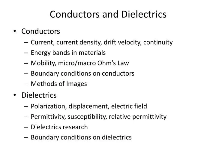
1. Conductors and Dielectrics • Conductors • Current, current density, drift velocity, continuity • Energy bands in materials • Mobility, micro/macro Ohm’s Law • Boundary conditions on conductors • Methods of Images • Dielectrics • Polarization, displacement, electric field • Permittivity, susceptibility, relative permittivity • Dielectrics research • Boundary conditions on dielectrics

2. Conductors and Dielectrics • Polarization • Static alignment of charge in material • Charge aligns when voltage applied, moves no further • Charge proportional to voltage • Conduction • Continuous motion of charge through material • Enters one side, exits another • Current proportional to voltage • Real-world materials • Plastics, ceramics, glasses -> dielectrics (maybe some conductivity) • Metals -> conductors, semiconductors, superconductors • Cement, Biosystems -> Both (water high dielectric, salt conductivity)

3. n Current and current density • Basic definition of current C/s = Amps • Basic current density (J perp. surface) • Vector current density

4. Current density and charge velocity • Basic definition of current • Combining with earlier expression • Gives current density

5. Charge and current continuity • Current leaving any closed surface is time rate of change of charge within that surface • Using divergence theorem on left • Taking time derivative inside integral • Equating integrands Qi(t)

6. Example – charge and current continuity • Given spherically symmetric current density • Current increasing from r = 5m to r= 6m at t=1s • Current density from continuity equation • Charge density ρ integral w.r.t. time • Drift velocity is thus ^^ Why is current increasing ? <<Some central repulsive force!

7. Energy Band Structure in Three Material Types • Discrete quantum states broaden into energy bands in condensed materials with overlapping potentials • Valence band – outermost filled band • Conduction band – higher energy unfilled band • Band structure determines type of material • Insulators show large energy gaps, requiring large amounts of energy to lift electrons into the conduction band. When this occurs, the dielectric breaks down. • Conductors exhibit no energy gap between valence and conduction bands so electrons move freely • Semiconductors have a relatively small energy gap, so modest amounts of energy (applied through heat, light,oran electric field) may lift electrons from valence to conduction bands.

8. Free electrons are accelerated by an electric field. The applied force on an electron of charge Q = -e is But in reality the electrons are constantly bumping into things (like a terminal velocity) so they attain an equilibrium or drift velocity: where eis the electron mobility, expressed in units of m2/V-s. The drift velocity is used in the current density through: So Ohm’s Law in point form (material property) With the conductivity given as: S/m (electrons/holes) Ohm’s Law (microscopic form) S/m (electrons)

9. Ohm’s Law (macroscopic form) • For constant electric field • Ohm’s Law becomes • Rearranging gives • Or • Variation with geometry • Conductance vs. Resistance

10. Ohm’s Law example 1 • Checking ohms law microscopic form • Mobility of copper is 0.0032 m2/V-s • Charge density

11. Ohm’s Law example 2

12. Boundary conditions for conductors • No electric field in interior • Otherwise charges repel to the surface • No tangential electric field at surface • Otherwise charges redistribute along surface • Normal electric field at surface • Displacement Normal equals Charge Density (Gauss’s Law)

13. or Over the rectangular integration path, we use To find: dielectric n These become negligible as h approaches zero. Therefore conductor More formally: Boundary Condition for Tangential Electric Field E

14. Gauss’ Law is applied to the cylindrical surface shown below: dielectric This reduces to: as h approaches zero n Therefore s conductor More formally: Boundary Condition for the Normal Displacement D

15. Tangential E is zero At the surface: Normal D is equal to the surface charge density Summary

16. Example - Boundary Conditions for Conductors • Potential given by • Potential at (2,-1,3) is 300 V. Also 300 V along entire surface where • Thus we can “insert” conductor in region provided the conductor follow hyperbola • The Electric Field is at all times normal to conducting surface • Electric field at point 2,-1,3) • Ex = -400 V/m, Ey = -200 V/m • Down and to left

17. Example – Streamlines of Electric Field • Slope of line equals electric field ratio • Rearranging • Evaluate at P(2,-1,3) -2

18. Boundary condition example (from my phone)* * www.mathstudio.net

19. The Theorem of Uniqueness states that if we are given a configuration of charges and boundary conditions, there will exist only one potential and electric field solution. In the electric dipole, the surface along the plane of symmetry is an equipotential with V = 0. The same is true if a grounded conducting plane is located there. So the boundary conditions and charges are identical in the upper half spaces of both configurations (not in the lower half). In effect, the positive point charge images across the conducting plane, allowing the conductor to be replaced by the image. The field and potential distribution in the upper half space is now found much more easily! Method of Images

20. Each charge in a given configuration will have its own image Forms of Image Charges

21. Want to find surface charge density on conducting plane at the point (2,5,0). A 30-nC line of charge lies parallel to the y axis at x=0, z = 3. First step is to replace conducting plane with image line of charge -30 nC at z = -3. Example of the Image Method

22. Vectors from each line charge to observation point: Electric Fields from each line charge Add both fields to get: (x component cancels) Example of the Image Method (continued) -

23. Electric Field at P is thus: Displacement is thus Charge density is n D Example of the Image Method (continued)

24. Image Method using Potentials • Conducting plane at x = 4 with vertical wire in front. • Potential for wire in front at x = 6, y=3: • Boundary condition for wire in front at x = 6, y=3: • Boundary condition for image wire in back at x=2, y=3:

25. Image Method using Potentials (cont) • Total potential becomes • At point (7,-1,5) gives • To get electric field must write V(ρ) as V(x,y) and take gradient

26. Dielectrics • Material has random oriented dipoles • Applied field aligns dipoles (negative at (+) terminal, positive at (-) terminal • Effect is to cancel applied field, lower voltage • OR, increase charge to maintain voltage • Either increases capacitance C= Q/V

27. Review Dipole Moment • Define dipole moment • Potential for dipole • Written in terms of dipole moment and position • Dipole moment determines “strength” of polar molecule amount of charge (Q) and offset (d) of charge

28. Introducing an electric field may increase the charge separation in each dipole, and possibly re-orient dipoles so that there is some aggregate alignment, as shown here. The effect is small, and is greatly exaggerated here! E The effect is to increase P. n = charge/volume p = polarization of individual dipole P = polarization/volume Polarization as sum of dipole moments (per volume)

29. E Polarization near electrodes positive • From diagram • Excess positive bound charge near top negative electrode • Excess negative bound charge near bottom positive electrode • Rest of material neutral • Excess charge in bound (red) volumes • Writing in terms of polarization • Writing similar to Gauss’s law (Note dot product sign, outward normal leaves opposite charge enclosed) - - - - - - - - - - - - - - - - neutral negative + + + + + + + + + + + + +

30. E Combining total, free, and bound charge positive • Total, free, and bound charge • Total • Free • Bound • Combining - - - - - - - - - - - - - - - - neutral negative + + + + + + + + + + + + +

31. D, P, and E in Dielectric • D continuous • Polarization increases • E decreases • C/m2

32. Bound Charge: Total Charge: Free Charge: Charge Densities Taking the previous results and using the divergence theorem, we find the point form expressions:

33. A stronger electric field results in a larger polarization in the medium. In a linear medium, the relation between P and E is linear, and is given by: where e is the electric susceptibility of the medium. We may now write: where the dielectric constant, or relative permittivity is defined as: Leading to the overall permittivity of the medium: where Electric Susceptibility and the Dielectric Constant

34. In an isotropic medium, the dielectric constant is invariant with direction of the applied electric field. This is not the case in an anisotropic medium (usually a crystal) in which the dielectric constant will vary as the electric field is rotated in certain directions. In this case, the electric flux density vector components must be evaluated separately through the dielectric tensor. The relation can be expressed in the form: Isotropic vs. Anisotropic Media

35. Permittivity of Materials • Typical permittivity for various solids and liquids. • Teflon – 2 • Plastics - 3-6 • Ceramics 8-10 • Titanates>100 • Acetone 21 • Water 78 • Actual dielectric “constant” varies with: • Temperature • Direction • Field Strength • Frequency • Real & Imaginary components

36. Variation with frequency • Charge polarization due to: • Ionic (low frequency) • Orientation (medium, microwave) • Atomic (IR) • Electronic (Visible, UV) • Dielectric relaxation • As frequency is raised, molecule can no longer “track”. • Real permittivity decreases and imaginary permittivity peaks • In medium and microwave range • Rotation, reorientation, etc >> • Modeling: • Permittivity & impedance diagrams. • Statistical relaxation functions (Debye, Cole Davidson).

37. Application to Polymer Composites • Dielectric Permittivity in Epoxy Resin 10Hz -10 MHz • Polar-group rotation in epoxy resin. • Low-frequency range 10 Hz – 10 MHz. • Permittivity-loss transition at 1 MHz, at –4°C. • Transition frequency increases with temperature. www.msi-sensing.com

38. Dielectric Permittivity in Epoxy Resin 1 MHz -1 GHz • Aerospace resin Hexcel 8552. • High frequency range 1 MHz – 1 GHz. • Temperature constant 125°C, transition decreases with cure. • TDR measurement method. www.msi-sensing.com

39. Permittivity in Epoxy Resin during Complete Cure Cycle www.msi-sensing.com

40. Application to cement hydration • Cement Conductivity - Variation with Cure • Imaginary counterpart of real permittivity (’’). • Multiply by  to remove power law (o’’). • Decrease in ion conductivity, growth of intermediate feature with cure • Frequency of intermediate feature does not match permittivity www.msi-sensing.com

41. Cement Cure -Dielectric Relaxation Model Requirements: • Provide free-relaxation, two intermediate-frequency relaxations • Provide conductivity and electrode polarization Debye for free & medium. Cole-Davidson for low. (literature, biosystems) Combined 9 variables fit over entire range, real & imaginary, 2-stage fit, f = 8.2 ps www.msi-sensing.com

42. Cement Cure - Model Fitting • Fits permittivity – both low and free relaxation. • Fits conductivity – both medium and free relaxation. • Fits permittivity polarization. • Fits conductivity baseline. www.msi-sensing.com

43. Other applications • Other Applications • Bio • Liquid Crystal • Composite polymers • Titanates • Wireless characterization • MRI dyes • Ground water monitoring • Oil Drilling fluid characterization (GPR)

44. Since E is conservative, we setup line integral straddling both dielectrics: Left and right sides cancel, so Leading to Continuity for tangential E Boundary Condition for Tangential Electric Field E And Discontinuity for tangential D E same, D higher in high permittivity material

45. n Apply Gauss’ Law to the cylindrical volume straddling both dielectrics s Flux enters and exits only through top and bottom surfaces, zero on sides Boundary Condition for Normal Displacement D Leading to Continuity for normal D (for ρS = 0) And Discontinuity for normal E D same. E lower in high permittivity material

46. Bending of D at boundary • Boundary conditions • DN continuous • Trigonometry • Eliminating DN high low

47. Example • Teflon εr = 2.1 • Displacement and Polarization outside • Displacement and Polarization inside • At boundary D is continuous, so inside

48. Example (continued) • Polarization up, E field down, D maintains continuity

49. Example

50. Quiz 2 – Problem 4.21