Microscopie en champ lointain par tomographie optique par diffraction

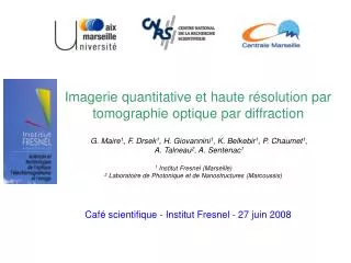
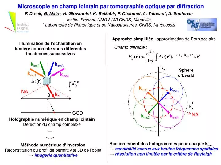
1. kinc3 kinc2 x ky y Sphère d’Ewald kinc1 kinc4 z (r) kinc1 kinc3 NA kd  kx CCD NA kinc2 kinc4 Microscopie en champ lointain par tomographie optique par diffraction F. Drsek, G. Maire,H. Giovannini,K. Belkebir, P. Chaumet, A. Talneau*, A. Sentenac Institut Fresnel, UMR 6133 CNRS, Marseille* Laboratoire de Photonique et de Nanostructures, CNRS, Marcoussis Approche simplifiée : approximation de Born scalaire Illumination de l’échantillon en lumière cohérente sous différentes incidences successives Champ diffracté : Holographie numérique en champ lointain Détection du champ complexe Raccordement des hologrammes pour chaque kinc → sensibilité accrue aux hautes fréquences spatiales → résolution non limitée par le critère de Rayleigh Méthode numérique d’inversion Reconstitution duprofil de permittivité 3D de l’objet → imagerie quantitative

2. kinc E qq µm résine 100 nm Si 633 nm Imagerie quantitative → profil de permittivité Montage optique en réflexion → adapté aux échantillons à forts contrastes d’indice Inversion numérique rigoureuse (gradients conjugués…) → diffusion multiple, forts contrastes d’indice Echantillons actuels 2D : Champs diffractés théoriques et expérimentaux Amplitude théorie expérience log(amplitude diffractée) (u.a.) Validation du montage en profilométrie  (°) Inversion par TF : limité à Born et aux approches perturbatives AFM Phase théorique (°) Phase expérimentale (°) Tomographie  (°)  (°)