CS 430/536 Computer Graphics I B-Splines and NURBS Week 5, Lecture 9

1. CS 430/536Computer Graphics IB-Splines and NURBSWeek 5, Lecture 9 David Breen, William Regli and Maxim Peysakhov Geometric and Intelligent Computing Laboratory Department of Computer Science Drexel University http://gicl.cs.drexel.edu

2. Outline • Types of Curves • Splines • B-splines • NURBS • Knot sequences • Effects of the weights

3. Splines • Popularized in late 1960s in US Auto industry (GM) • R. Riesenfeld (1972) • W. Gordon • Origin: the thin wood or metal strips used in building/ship construction • Goal: define a curve as a set of piecewise simple polynomial functions connected together

4. Natural Splines • Mathematical representation of physical splines • C2 continuous • Interpolate all control points • Have Global control (no local control)

5. B-splines: Basic Ideas • Similar to Bézier curves • Smooth blending function times control points • But: • Blending functions are non-zero over only a small part of the parameter range (giving us local support) • When nonzero, they are the “concatenation” of smooth polynomials. (They are piecewise!)

6. B-spline: Benefits • User defines degree • Independent of the number of control points • Produces a single piecewise curve of a particular degree • No need to stitch together separate curves at junction points • Continuity comes for free

7. B-splines • Defined similarly to Bézier curves • pi are the control points • Computed with basis functions (Basis-splines) • B-spline basis functions are blending functions • Each point on the curve is defined by the blending of the control points (Biis the i-th B-spline blending function) • Bi is zero for most values of t!

8. B-splines: Cox-deBoor Recursion • Cox-deBoor Algorithm: defines the blending functions for spline curves (not limited to deg 3) • curves are weighted avgs of lower degree curves • Let denote the i-th blending function for a B-spline of degree d, then:

9. B-spline blending functions B-spline Blending Functions • is a step function that is 1 in the interval • spans two intervals and is a piecewise linear function that goes from 0 to 1 (and back) • spans three intervals and is a piecewise quadratic that grows from 0 to 1/4, then up to 3/4 in the middle of the second interval, back to 1/4, and back to 0 • is a cubic that spans four intervals growing from 0 to 1/6 to 2/3, then back to 1/6 and to 0 Pics/Math courtesy of Dave Mount @ UMD-CP

10. B-spline Blending Functions:Example for 2nd Degree Splines • Note: can’t define a polynomial with these properties (both 0 and non-zero for ranges) • Idea: subdivide the parameter space into intervals and build a piecewise polynomial • Each interval gets different polynomial function Pics/Math courtesy of Dave Mount @ UMD-CP

11. B-spline Blending Functions:Example for 3rd Degree Splines • Observe: • at t=0 and t=1 just four of the functions are non-zero • all are >=0 and sum to 1, hence the convex hull property holds for each curve segment of a B-spline 1994 Foley/VanDam/Finer/Huges/Phillips ICG

12. B-splines: Knot Selection • Instead of working with the parameter space , use • The knot points • joint points betweencurve segments, Qi • Each has a knot value • m-1 knots for m+1 points 1994 Foley/VanDam/Finer/Huges/Phillips ICG

13. Uniform B-splines:Setting the Options • Specified by • m+1control points, P0 … Pm • m-2cubic polynomial curve segments, Q3…Qm • m-1 knot points, t3 … tm+1 • segmentsQi of the B-spline curve are • defined over a knot interval • defined by 4 of the control points, Pi-3 … Pi • segments Qi of the B-spline curve are blended together into smooth transitions via (the new & improved) blending functions

14. Example: Creating a B-spline • m = 9 • 10 control points • 8 knot points • 7 segments 1994 Foley/VanDam/Finer/Huges/Phillips ICG

15. B-spline: Knot Sequences • Even distribution of knots • uniform B-splines • Curve does not interpolate end points • first blending function not equal to 1 at t=0 • Uneven distribution of knots • non-uniform B-splines • Allows us to tie down the endpoints by repeating knot values (in Cox-deBoor, 0/0=0) • If a knot value is repeated, it increases the effect (weight) of the blending function at that point • If knot is repeated d times, blending function converges to 1 and the curve interpolates the control point

16. B-splines: Cox-deBoor Recursion • Cox-deBoor Algorithm: defines the blending functions for spline curves (not limited to deg 3) • curves are weighted avgs of lower degree curves • Let denote the i-th blending function for a B-spline of degree d, then:

17. Creating a Non-UniformB-spline: Knot Selection • Given curve of degree d=3, with m+1 control points • first, create m+d knot values • use knot values (0,0,0,1,2,…, m-2, m-1,m-1,m-1) (adding two extra 0’s and m-1’s) • Note • Causes Cox-deBoor to giveadded weight in blending to thefirst and last points when t isnear tmin and tmax Pics/Math courtesy of G. Farin @ ASU

18. B-splines: Multiple Knots • Knot Vector{0.0, 0.0, 0.0, 3.0, 4.0, 5.0, 6.0, 7.0} • Several consecutive knots get the same value • Changes the basis functions! From http://devworld.apple.com/dev/techsupport/develop/issue25/schneider.html

19. B-spline Summary

20. Watching Effects of Knot Selection 0 0 1 2 3 4 5 6 7 8 9 • 9 knot points (initially) • Note: knots are distributed parametrically based on t, hence why they “move” • 10 control points • Curves have as many segments as they have non-zero intervals in u degree of curve Pics/Math courtesy of G. Farin @ ASU

21. B-splines: Local Control Property • Local Control • polynomial coefficients depend on a few points • moving control point (P4) affects only local curve • Why: Based on curve def’n, affected region extends at most 2 knot points away 1994 Foley/VanDam/Finer/Huges/Phillips ICG

22. B-splines: Local Control Property Recorded from: http://heim.ifi.uio.no/~trondbre/OsloAlgApp.html

23. B-splines: Convex Hull Property • The effect of multiple control points on a uniform B-spline curve 1994 Foley/VanDam/Finer/Huges/Phillips ICG

24. B-splines: Continuity • Derivatives are easy for cubics • Derivative:Easy to show C0 ,C1 ,C2

25. B-splines: Setting the Options • How to space the knot points? • Uniform • equal spacing of knots along the curve • Non-Uniform • Which type of parametric function? • Rational • x(t), y(t), z(t) defined as ratio of cubic polynomials • Non-Rational

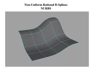
26. NURBS • At the core of several modern CAD systems • I-DEAS, Pro/E, Alpha_1 • Describes analytic and freeform shapes • Accurate and efficient evaluation algorithms • Invariant under affine and perspective transformations U of Utah, Alpha_1

27. Benefits of Rational Spline Curves • Invariant under rotation, scale, translation, perspective transformations • transform just the control points, then regenerate the curve • (non-rationals only invariant under rotation, scale and translation) • Can precisely define the conic sections and other analytic functions • conics require quadratic polynomials • conics only approximate with non-rationals

28. NURBS Non-uniform Rational B-splines: NURBS • Basic idea: four dimensional non-uniform B-splines, followed by normalization via homogeneous coordinates • If Pi is [x, y, z, 1], results are invariant wrt perspective projection • Also, recall in Cox-deBoor, knot spacing is arbitrary • knots are close together, influence of some control points increases • Duplicate knots can cause points to interpolate • e.g. Knots = {0, 0, 0, 0, 1, 1, 1, 1} create a Bézier curve

29. Rational Functions • Cubic curve segmentswhereare all cubic polynomials with control points specified in homogenous coordinates, [x,y,z,w] • Note: for 2D case,

30. Rational Functions: Example • Example: • rational function: a ratio of polynomials • a rational parameterization in u of a unit circle in xy-plane: • a unit circle in 3D homogeneouscoordinates:

31. NURBS: Notation Alert • Depending on the source/reference • Blending functions are either or • Parameter variable is either u or t • Curve is either C or P or Q • Control Points are either Pior Bi • Variables for order, degree, number of control points etc are frustratingly inconsistent • k, i, j, m, n, p, L, d, ….

32. NURBS: Notation Alert • If defined using homogenous coordinates, the 4th (3rd for 2D) dimension of each Pi is the weight • If defined as weighted euclidian, a separate constant wi, is defined for each control point

33. NURBS • A d-th degree NURBS curve C is def’d as:Where • control points, • d-th degree B-spline blending functions, • the weight, wi, for control point Pi(when all wi=1, we have a B-spline curve)

34. Observe: Weights Induce New Rational Basis Functions, R • Setting:Allows us to write:Where are rational basis functions • piecewise rational basis functions on • weights are incorporated into the basis fctns

35. Geometric Interpretation of NURBS • With Homogeneous coordinates, a rational n-D curve is represented by polynomial curve in (n+1)-D • Homogeneous 3D control points are written as:in 4D where • To get , divide by wi • a perspective transform with center at the origin • Note: weights can allow final curve shape to go outside the convex hull (i.e. negative w)

36. NURBS: Examples • Unif. Knot Vector • Non-Unif. Knot Vector {0.0, 1.0, 2.0, 3.0, 4.0, 5.0, 6.0, 7.0} {0.0, 1.0, 2.0, 3.75, 4.0, 4.25, 6.0, 7.0} From http://devworld.apple.com/dev/techsupport/develop/issue25/schneider.html

37. NURBS: Examples • Knot Vector{0.0, 0.0, 0.0, 3.0, 4.0, 5.0, 6.0, 7.0} • Several consecutive knots get the same value • Bunches up the curve and forces it to interpolate From http://devworld.apple.com/dev/techsupport/develop/issue25/schneider.html

38. NURBS: Examples • Knot Vector{0.0, 1.0, 2.0, 3.0, 3.0, 5.0, 6.0, 7.0} • Several consecutive knots get the same value • Bunches up the curve and forces it to interpolate • Can be done midcurve From http://devworld.apple.com/dev/techsupport/develop/issue25/schneider.html

39. The Effects of the Weights • wi of Pi effects only the range [ui, ui+k+1) • If wi=0 then Pi does not contribute to C • If wi increases, point B and curve C are pulled towardPi and pushed away from Pj • If wi decreases, point B and curve C are pushed away from Pi and pulled toward Pj • If wi approaches infinity thenB approaches 1 and Bi -> Pi , if u in [ui, ui+k+1)

40. The Effects of the Weights • Increased weight pulls the curve toward B3 From http://devworld.apple.com/dev/techsupport/develop/issue25/schneider.html

41. Programming assignment 3 • Input PostScript-like file containing polygons • Output B/W XPM • Implement viewports • Use Sutherland-Hodgman intersection for polygon clipping • Implement scanline polygon filling. (You cannot use flood filling)