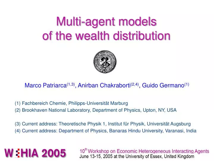
Multi-agent models of the wealth distribution

1. Multi-agent modelsof the wealth distribution Marco Patriarca(1,3), Anirban Chakraborti(2,4), Guido Germano(1) (1) Fachbereich Chemie, Philipps-Universität Marburg (2) Brookhaven National Laboratory, Department of Physics, Upton, NY, USA (3) Current address: Theoretische Physik 1, Institut für Physik, Universität Augsburg (4) Current address: Department of Physics, Banaras Hindu University, Varanasi, India

2. Motivation Kinetic multi-agents models can reproduce some general relevant features of wealth distributions such as: • zero limit at very small wealth • a mode larger than zero • an exponential law at low and intermediate wealth • a power law at large wealth (first observed by Pareto) • a fraction of richest agents of a few percent from A. Dragulescu and V. M. Yakovenko, Eur. Phys. J. B 17, 723 (2000). from H. Aoyama, W. Souma, and Y. Fujiwara, Physica A 324, 352 (2003).

3. Overview of the talk • Generalities about kinetic multi-agent models: I. The basic model II. The model with global saving propensity 0  (0,1) III. The model with individual saving propensities  i  (0,1) • The richest agents: influence of saving propensity on wealth, and power law as overlap of exponentials • Some examples of realistic distributions

4. 3 1 2 j 4 x i N-2 N-1 N Wealth is measured with a single variable x, e.g. in a currency unit. Money is in fact a well defined quantity that can be used for measuring all economic goods which contribute to wealth.

5. I. Basic Model [1,2,3] • Nagents with wealth {xi}, i = 1, ..., N • At every time step t two agents k and jare extracted at random • x is redistributed at random between agents kand j (r = random number between 0 and 1) • Time evolution is carried out until equilibrium is reached [1]A. Dragulescu and V. M. Yakovenko, Statistical mechanics of money, Eur. Phys. J. B 17 (2000) 723. [2]E. Bennati, Un metodo di simulazione statistica nell'analisi della distribuzione del reddito, Rivista Internazionale di Scienze Economiche e commerciali (1988) 735; E. Bennati, Il metodo Montecarlo nell'analisi economica, Rassegna di lavori dell'ISCO 4 (1993) 31. [3] J. Angle, The surplus theory of social stratification and the size distribution of personal wealth, in Proceedings of the Social Statistics Section of the American Statistical Association, 1983, p. 395; J. Angle, The surplus theory of social stratification and the size distribution of personal wealth, Social Forces 65 (1986) 293

6. Equilibrium distribution: The model is robust in that the corresponding Boltzmann (or Gibbs) distribution is obtained in different conditions: • Different initial distributions of x • Pairwise as well as multi-agent interactions • Constant as well as randomx • Random, first neighbour, as well as consecutive selection of the interacting agents • Various linear forms of x • Rapid convergence to equilibrium distribution also for a very small number of agents i.e. the Boltzmann distribution, where x is the average value of x.

7. II.Model with saving propensity  (0 <  < 1) [3,4,5] • Nagents with wealth {xi}, i = 1, ..., N • At every time step ttwo agents k and j are extracted at random • x is redistributed randomly between k and j , r = random number in (0,1) [3] A. Chakraborti, PhD Thesis. [4] A. Chakraborti, B. K. Chakrabarti, Eur. Phys. J. B 17, 167 (2000). [5] A. Chakraborti, Int. J. Mod. Phys. C 13, 1315 (2002)

8. Equilibrium distribution The equilibrium distribution is a Gamma-distribution: where ‹x› is the average x and anthe normalization constant,

10. III. Model with individual saving propensities i(0 < i< 1) [1,2] • Nagents with wealth {xi} and saving propensities {i} • At every time step textract randomly two agents k and j • Wealth is then redistributed randomly between k and jaccording to a money-conserving stochastic dynamics

11. N=100 N=1000 N=10 x - 2 Equilibrium distribution

12. The Boltzmann equationapproach[1,2,3,4] • The Boltzmann equation approach to multi-agent systems can predict many features of the wealth distribution. • For instance, the power law for the distribution function is -2 [1,2,3,4]. • The first 2 moments are identical to those of the Gamma distribution [1]. • One can also predict the asymptotic time dependence [4]. • Also, precious information about the role of agents with a high given value of saving propensity can be obtained. [1] Das, Yarlagadda, A distribution function analysis of wealth distribution, URL arXiv:cond-mat/0310343. [2] P. Repetowicz, S. Hutzler, P. Richmond, Dynamics of Money and Income Distributions, Phisica A, in press [3] A. Chatterjee, B. K. Chakrabarti, R. B. Stinchcombe, Master equation for a kinetic model of trading market and its analytic solution, cond-mat/0501413; Analyzing money distributions in ‘ideal gas’ models of marketsphysics/0505047 [4]S. Ispolatov, P. Krapivsky, S. Redner, Wealth distributions in asset exchange models,Eur. Phys. J. B 2, 267 (1998).

13. 10 1 x 0.1 0.01 0.1 0.2 0.3 0.4 0.5 0.6 0.7 0.8 0.9 1  Correlation between wealth and saving propensity • In models with individual saving propensities there is a correlation between • the individual saving propensity n and the corresponding wealth xn. • This happens quite generally, for random as well as deterministic assignment • of n , for power or nonpower laws, for all distributions of n. • dots are single agents, • the continuous • line is the average • ‹x›~ 1 / (1– ). .

14. Richer agents remain richer(only a poor agent’s wealth varies appreciably during a trade) • Rich agents will never risk all their money: they have a large saving propensity ( ≈ 1) and therefore a low effective temperature T ≈ (1-  ) • Thus they risk only a small amount of money in a trade • This is shown by the small width of the x(t+1)-x(t) map at large values of x.

15. Thermodynamical modelling T1 T2 N = N1 + N2 + N3 N1have saving propensity 1, N2have saving propensity 2 N3have saving propensity 3 xi ~ 1 / (1– i) Di = 2 (1 + 2 i) / (1  i) Ti = 2 xi/ Di = xi (1  i) / (1 + 2 i) D1 D2 T3 D3

16. Influence of -cutoff Example of a system with 100 000 agents and a uniform -distribution from  =0 up to =M. The wealth distribution ends at a cutoff determined by the cutoff of the saving propensity distribution. The richest agent has the highest saving propensity, as follows from the x-correlation.

17. Influence of -cutoff The tail of the -distribution can influence the tail of the wealth distribution revealing the single-agent structure at the highest .

18. Toward a more realistic distribution Following a suggestion by A. Chatterjee, B. K. Chakrabarti, and S. S. Manna [Physica Scripta T106, 36 (2003)] one can prepare a -distribution with a small fraction of agents with uniformly distributed  and the rest with a fixed . Here is an example with 99% of agents with =0.2 and 1% with uniformly distributerd :

19. Conclusions • Subsystems with a given irelax to exponential (Gamma) distributions • They behave as open, coupled subsystems with their own temperature Ti and effective dimension Di . • A power law is obtained naturally from the superpositions of such distributions. • Realistic shapes of wealth distributions can be obtained from suitable • -distributions. Acknowledgments Marco Patriarca’s work on this subject started at the Laboratory of Computational Engineering, Helsinki University of Technology, under support of the Academy of Finland, Research Centre for Computational Science and Engineering, project nr. 44897 (Finnish Centre for Excellence Program 2000-2005). Anirban Chakraborti’s work at Brookhaven National Laboratory was carried out under Contract nr. DE-AC02-98CH10886, Division of Material Science, U.S. Department of Energy.