Download
1 / 58
580 likes | 638 Views
Network Layer. Provides for the transparent transfer of data between transport entities. Responsible for: Establishing, Maintaining, Terminating connections Across the intervening communication facility. Routing packets within subnet, Congestion and deadlock problems,

E N D
Network Layer Provides for the transparent transfer of data between transport entities. Responsible for: • Establishing, • Maintaining, • Terminating connections Across the intervening communication facility. • Routing packets within subnet, • Congestion and deadlock problems, • Subnet-host interface?
Network Layer (cont.) Service Provided: Issue Connection- Connectionless oriented Initial setup Required Not possible Destination Only needed Needed on address during setup every packet Packet Guaranteed Not guaranteed sequencing Done by Done by Error network layer transport layer control (e.g., subnet) (e.g., hosts)
Network Layer (cont.) Issue Connection- Connectionless oriented Flow Provided by Not provided control network layer by network layer Is option negotiation Yes No possible? Are connection Yes No identifiers used? Summary of the major differences between connection-oriented and connectionless service.
E-mail FTP … TCP IP ATM Data link Physical Running TCP/IP over an ATM subnet
Virtual Circuits vs Datagrams • Trade-off between IMP memory, space and bandwidth • Virtual circuits (used in SNA) • Attractive for interactive terminal environment • Packet contains circuit # vs full destination address • Problem: If IMP fails and loses its memory, then every thing is lost. • Error control and sequence control (handled by data link layer)
Virtual Circuits vs Datagrams (cont.) • Datagrams (used in DECNET, ARPANET) • Allow IMPs to balance load • Host (transport layer) inserts error control and sequence control.
Connectionless Connection-oriented Circuit setup Addressing State information Routing Effect of node failures Congestion control Complexity Suited for Not possible Each packet contains the full source and destination address Subnet does not hold state information Each packet is routed independently None, except for packets lost during the crash Difficult In the transport layer Connection-oriented and connectionless service Required Each packet contains a short vc number Each established vc requires subnet table space Route chosen when vc is setup; all packets follow this route All vcs that passed through the failed equipment are terminated Easy if enough buffers can be allocated in advance for each vc set up In the network layer Connection-oriented service Comparison of datagram and virtual circuit subnets
H Host H 8 Simplex virtual circuits Originating at A 0 - ABCD 1 - AEFD 2 - ABFD 3 - AEC 4 - AECDFB B C H A D Originating at B 0 - BCD 1 - BAE 2 - BF H E F H H IMP Virtual Circuit Subnet (b) Eight virtual circuits through the subnet (a) Example subnet
Virtual Circuit Subnet (cont.) (c) IMP tables for the virtual circuits in (b)
Virtual circuit field Line H to A E to C C to D B to H A to E D to F F to B 4 3 1 2 0 0 0 packet Virtual Circuit Subnet (cont.) (d) The virtual circuit changes as a packet progresses
Routing Algorithms • Concern: • Correctness • Robustness • Simplicity • Fairness • Stability • Optimality Note: Trade-off between fairness and optimality.
Routing Algorithms (cont.) • 2 classes of routing algorithm • Nonadaptive • Adaptive • Centralized • Isolated • Distributed
Example packet-switched network 5 To node 3 2 3 1 2 3 4 5 6 1 = 2 4 4 4 4 2 1 = 3 4 4 4 3 5 2 = 5 5 5 4 1 2 5 = 5 5 5 4 4 3 4 = 6 6 5 5 5 5 5 = 5 2 3 2 1 6 From Node 1 2 1 1 4 5 Central Routing Directory
Example packet-switched network: Fixed routing Node 1 Directory Dest. Next node 2 2 3 4 4 4 5 4 6 4 Node 2 Directory Dest. Next node 1 1 3 3 4 4 5 4 6 4 Node 3 Directory Dest. Next node 1 5 2 2 4 5 5 5 6 5 Node 4 Directory Dest. Next node 1 1 2 2 3 5 5 5 6 5 Node 5 Directory Dest. Next node 1 4 2 4 3 3 4 4 6 6 Node 6 Directory Dest. Next node 1 5 2 5 3 5 4 5 5 5
B C 7 2 E F 2 3 2 3 A D 6 1 2 2 4 G H Dijkstra's Algorithm B (2,A) C (¥,-) 7 2 E (¥,-) F (¥,-) 2 3 2 3 A D (¥,-) 6 1 2 2 4 G (6,A) H (¥,-) Shortest path from A to D
B (2,A) C (9,B) 7 2 E (4,B) F (¥,-) 2 3 2 3 A D (¥,-) 6 1 2 2 4 G (6,A) H (¥,-) Dijkstra's Algorithm (cont.) B (2,A) C (9,B) 7 2 E (4,B) F (6,E) 2 3 2 3 A D (¥,-) 6 1 2 2 4 G (5,E) H (¥,-) Shortest path from A to D
B (2,A) C (9,B) 7 2 E (4,B) F (6,E) 2 3 2 3 A D (¥,-) 6 1 2 2 4 G (5,E) H (9,G) Dijkstra's Algorithm (cont.) B (2,A) C (9,B) 7 2 E (4,B) F (6,E) 2 3 2 3 A D (¥,-) 6 1 2 2 4 G (5,E) H (8,F) Shortest path from A to D
Dijkstra's Algorithm (cont.) B (2,A) C (9,B) 7 2 E (4,B) F (6,E) 2 3 2 3 A D(10,H) 6 1 2 2 4 G (5,E) H (8,F) Shortest path from A to D
Multipath Routing Advantage over shortest path routing: Possibility of sending different classes of traffic over different paths. e.g., Short packets routed via terrestrial lines, whereas a long file routed via satellite. Note: Disjoint paths improve reliability and performance.
Multipath Routing (cont.) First Choice A 0.63 A 0.46 A 0.34 H 0.50 A 0.40 A 0.34 H 0.46 H 0.63 I 0.65 K 0.67 K 0.42 Second Choice I 0.21 H 0.31 I 0.33 A 0.25 I 0.40 H 0.33 A 0.31 K 0.21 A 0.22 H 0.22 H 0.42 Third Choice H 0.16 I 0.23 H 0.33 I 0.25 H 0.20 I 0.33 K 0.23 A 0.16 H 0.13 A 0.11 A 0.16 Dest A B C D E F G H I - K L A B C D E G H F K I J L Routing Table for Node J
Centralized Routing • Adaptive routing scheme based on routing control center (RCC). • Use global information to optimize individual IMPs. • Lots of overhead. • Vulnerable to failure of RCC. • Timing problem during update. • Heavy traffic through RCC. • Advantage; Bursty traffic.
Isolated Routing • Adaptive, but fewer vulnerability problems than centralized routing. • Routing information is not passed among IMPs, but IMPs ``learn'' from past I/O schemes. • Hot potato -- IMP tries to get rid of packet quickly, by putting it on shortest output Q. • Backward learning -- use frame headers to pass information among IMP about history of packet.
Isolated Routing (cont.) • Delta routing -- hybrid between isolated and centralized. • Each IMP measures the cost of each line (i.e., some function of delay, Q length, utilization, etc) and periodically send a packet to the RCC giving these values. To A To H To I To K Queueing within the IMP
Flooding Every incoming packet is sent out on all outgoing lines except the one it arrived on. Note: Not practical in most applications. However, flooding produces shortest delay (if overhead is ignored) • Selective flooding • Random walk Static routing fixed tables. Each possible route is weighted
Flooding example (hop count=3) Assume that a packet is to be sent from node 1 to node 6.
Distance Vector Routing • Each IMP exchanges information with its neighbors. • Routing table in each IMP contains Distance or time to destination Destination Best line All IMPs in network
Distance Vector Routing (cont’d) New estimated delay from J A 0 12 25 40 14 23 18 17 21 9 24 29 I 24 36 18 27 7 20 31 20 0 11 22 33 H 20 31 19 8 30 19 6 0 14 7 22 9 K 21 28 36 24 22 40 31 19 22 10 0 9 Line A A I H I I H H I - K K A B C D E F G H I J K L 8 20 28 20 17 30 18 12 10 0 6 15 A B C D E G H F K I J L (a) Subnet JA delay = 8 10 12 6 (b) Input from A,I,H,K and the new routing table for J
Link State Routing • Discover its neighbors and learn their network addresses • Measure the delay or cost to each of its neighbors • Construct a packet telling all it has just learned • Send this packet to all other routers • Compute the shortest path to every other router
Routers H B D E D E G I H B G C A C F A I F N LAN Learning about the Neighbors • Send a special HELLO packet on each point -to point line • Two or more routers are connected by a LAN (a) Nine routers and a LAN (b) A graph model of (a)
Measuring Line Cost • Estimate delay of neighbors • Send special ECHO over line • Measure the roundtrip time and divide by 2 • Load consider?
2 A B C D E F B C Seq. Seq. Seq. Seq. Seq. Seq. 4 3 Age Age Age Age Age Age B 4 A 4 B 2 C 3 A 5 B 6 A D 1 6 E 5 C 2 D 3 F 7 C 1 D 7 5 7 F 6 E 1 F 8 E 8 E 8 F (a) A subnet (b) The link state packets for this subnet Building Link State Packets
Send flags ACK flags Source Seq. Age A C F A C F Data A F E C D 21 21 21 20 21 60 60 59 60 59 0 1 0 1 1 1 1 1 0 0 1 0 0 1 0 1 0 1 0 0 0 0 0 1 1 0 1 1 0 1 The packet buffer for router B Distributing the Link State Packets • Use flooding
Computing the Routes • Use Dijkstra’s Algorithm • OSPF Protocol (used in Internet)
Optimal Routing (a) A subnet (b) The sink tree for IMP B,using number of hops as metric
Flow-Based Routing Basic Idea: For a given line, if the capacity and average flow are known, it is possible to compute the mean packet delay on that line from queueing theory. The routing then reduces to finding the routing algorithm that produces the minimum average delay for the network.
Flow-Based Routing (cont.) Destination A 9 BA 4 CBA 1 DFBA 7 EA 4 FEA B 9 AB 8 CB 3 DFB 2 EFB 4 FB E 7 AE 2 BFE 3 CE 3 DCE 5 FE F 4 AEF 4 BF 2 CEF 4 DF 5 EF C 4 ABC 8 BC 3 DC 3 EC 2 FEC D 1 ABFD 3 BFD 3 CD 3 ECD 4 FD A B C D E F Source 20 B C 20 10 20 A D 20 10 20 E F 50 (a) A network with line capacity shown in Kbps (b) The traffic in packets/sec and the routing matrix
Flow-Based Routing (cont.) l (pkts/sec) 14 12 6 11 13 8 10 8 C (kbps) 20 20 10 20 50 10 20 20 mC (pkts/sec) 25 25 12.5 25 62.5 12.5 25 25 T (ms) 91 77 154 71 20 222 67 59 i 1 2 3 4 5 6 7 8 Line AB BC CD AE EF FD BF EC Analysis of the above network using a mean packet size of 800 bits. The reverse traffic (BA, CB, etc) is the same as the forward traffic
Hierarchical Routing Dest. Line hops Dest. Line hops 1A - - 1B 1B 1 1C 1C 1 2A 1B 2 2B 1B 3 2C 1B 3 2D 1B 4 3A 1C 3 3B 1C 2 4A 1C 3 4B 1C 4 4C 1C 4 5A 1C 4 5B 1C 5 5C 1B 5 5D 1C 6 5E 1C 5 1A - - 1B 1B 1 1C 1C 1 2 1B 2 3 1C 2 4 1C 3 5 1C 4 Region 1 Region 2 1B 2A 2B 1C 2D 1A 2C Hierarchical Table For 1A 5B 4A 5C 3B 3A 4B 4C 5A 5D 5E Region 3 Region 4 Region 5 Full Table For 1A
Routing For Mobile Hosts Wireless cell Home agent Mobile host Home LAN Foreign LAN WAN MAN A WAN to which LANs, MANs, and wireless cells are attached
Routing For Mobile Hosts (cont.) The registration procedure for mobile hosts: 1. Periodically, each foreign agent broadcast a packet announcing its existance and address. A newly arrived mobile host may wait for one of these messages, but if none arrives quickly enough, the mobile host can broadcast a packet saying: “Are there any foreign agents around?” 2. The mobile host registers with the foreign agent, giving its home address, current data link layer address, and some security information.
Routing For Mobile Hosts (cont.) 3. The foreign agent contacts the mobile host’s home agent and says: “One of your hosts is over here.” The message from the foreign agent to the home agent contains the foreign agent’s network address. It also includes the security information, to convince the home agent that the mobile host is really there. 4. The home agent examines the security information which contains a timestamp, to prove that it was generated within the past few seconds. If it is happy, it tells the foreign agent to proceed.
Routing For Mobile Hosts (cont.) 5. When the foreign agent gets the acknowledgement from the home agent, it makes an entry in its table and informs the mobile host that it is now registered.
Routing For Mobile Hosts (cont.) 1. Packet is sent to the mobile host’s home address 3. Sender is given foreign agent’s address 4. Subsequent packets are tunneled to the foreign agent 2. Packet is tunneled to the foreign agent Packet routing for mobile users
Broadcast Routing (cont.) • Source to send a packet to each destination. • Flooding. • Multidestination routing -- each packet contains a list of destinations. • Spanning tree -- copy an incoming packet onto all the spanning tree lines except the one it arrived on.
Traffic Control • Flow control e.g., Sliding window technique • Congestion control e.g., Managing input and output buffers at IMPs. • Packets may be discarded or • A choke packet sent. • Deadlocks e.g., No buffers are available.
Traffic Control (cont.) To 2 To 3 To 1 Node 4 To 5 Output Buffer Intput Buffer Input and Output Queues at node 4 To host
Traffic Control (cont.) 2 3 1 6 4 5 Host The interaction of queues in a packet-switching network
The effects of congestion throughput (packets delivered) (a) Throughput