NUMERICAL ANALYSIS OF SIMPLIFIED RELIC-BIREFRINGENT GRAVITATIONAL WAVES

1. NUMERICAL ANALYSIS OF SIMPLIFIED RELIC-BIREFRINGENT GRAVITATIONAL WAVES Rafael de la Torre Dr. David Garrison 3/29/10

2. In The Beginning …. • Standard model of the universe (Big Bang) • Originally discovered by Edwin Hubble’s observations of distant galaxies • Red-shifted in all directions = accelerating away • Decades of supporting evidence • Confirmation of Hubble’s observations from various sources • Cosmic Microwave Background (CMB) observations

3. Standard Model

4. Big “Problems” • Horizon and Smoothness Problems: The Universe exhibits large-scale homogeneity that shouldn’t exist • Flatness Problem: The Universe shouldn’t be ~flat today

5. Inflation Theory • Solves problems with standard model • Proposed by MIT PhysicistAlan Guth in 1980 • Extremely rapid expansion of the universe in a very short time span (~10-35 to ~10-32 s) Horizon and Smoothness Problems Flatness Problem

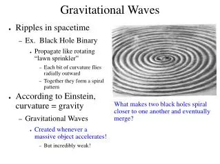
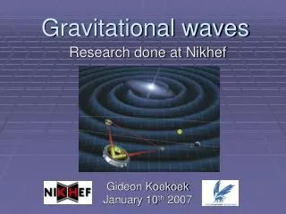
6. Gravitational Waves • Prediction of Einstein’s General Relativity • Space-Time curved by mass • Larger mass corresponds to greater curvature • Einstein’s equations can be written as wave equations using adequate assumptions • Very large mass-energy objects in motion can produce “ripples” in space-time • Ripples = Gravity Waves (GWs) • Possible Sources Include: • Black holes, massive/dense stars • Very early universe Relic GWs are remnants of the exponential inflation of the very early universe

7. Gravitational Spectrum

8. Relic GWs • Possibly associated with cosmological structure formation • Leptogenesis • GRMHD turbulence • Recent work by Alexander, et al. adds potential Quantum Gravitation effects • Inclusion of QG terms predicts very small anisotropies in space-time during early universe • Anisotropies produce Birefringent (BRF) GWs with different polarities

9. Detection • Relic GW theory suggests a CMB analog may exist for gravitational radiation • Cosmic Gravitational Wave Background (CGWB) • Detecting relic-BRF GWs would provide evidence of inflation and QG effects • GW spectrum is needed to focus detectors on certain amplitude vs. frequency regions

10. Relic GW Spectrum • Relic GWs result in tensor perturbations to the ST metric • Spectrum determined using QM approach • Tensor perturbations become operators in Quantum-Gravitational expectation function • Computation of spectrum is only required at some conformal time () during inflation Mode Function is primary variable to determine! Mean-square amplitude of spectrum

11. Mode Functions • Composed of GW equation and “effective” scale factor • Scale factor and effective scale factor have the following form during inflation • GW equation is key to determine mode function! • Given by equation for 1-D Harmonic oscillator for

12. Standard and Simplified BRF Relic GWs

13. Red-shift of RMS Amplitude • Spectral amplitude at inflation is red-shifted for sub-Hubble radius wave lengths to any time since • Method developed by Grischuk for standard GW spectrum • Red-shift is function of scale factors at different “breakpoints” • Breakpoints correspond to transition between different eras • Red-shift during each era determined by general relation

14. Variable Properties • Frequency & wave number - 1e-20 < < 1e+10 • Low-frequency limit corresponds to wave lengths > current Hubble radius • High-frequency limit established from relationship • Power-law expansion parameter -  = -2 and -1.9 • Theoretical restriction - 1+  < 0 • Values chosen encompass expected range • -2 Corresponds to de Sitter Universe (No Matter, + ) • -1.9 incorporates slow-roll approximation (falls within this range) • BRF Parameter -  < 1e-05 • Composed of QG and string theory parameters • Values > than this result in non-linear Veff • Conformal Time - ||< 1e-18 • Due to numerical instabilities in high frequency regime • Results from constraint k   << 1

15. Numerical approach • Used Numerical routines available in MATLAB • Applied built-in Bessel & Gamma functions • Imported and modified special complex Kummer & Gamma function modules from user community • Evolved particular solutions of GW equations using variable constraints • Calculated mode function and spectrum at initial conformal time for each step through GW equations • Red-shifted initial spectrum using Grishchuk’s method depending on values of  • Plotted resulting spectrum and differences between models • Validity check • BRF GW algorithms numerically computed with theta = 0 to compare against standard values • Compared results to theoretical approximations where possible

16. Relic GW SpectrumRMS Amplitude vs Frequency Spectrum for  = -2 Space Based LISA Ground Based LIGO I LIGO II Pulsar Timing (RMS- Amplitude) Spectrum for  = -1.9  Standard vs BRF for  = -1.9  Standard vs BRF for  = -2 Planck scale (Frequency)

17. Conclusions • GW spectrum for simplified BRF GWs does not appear to be significantly different than the standard GW spectrum at the present time • Indicates that BRF GW ~ Standard GW for k|| << 1 during instant of GW creation • If BFR GW were created, they may not be distinguishable unless  and k|| are different than assumptions • Review of general BRF analytical solutions imply limit on conformal time of GW creation (at least for RH wave) • k|| < ½ so ||< 5e-15

18. Forward Work • Apply red-shift for accelerating Universe as proposed by Zhang, et al. for completeness • Examine numerical solution to general BRF GW ODE • Variable  • Examine non-linear behavior and implications for  > 1e-05 • Determine Spectrum at 3 minutes to support GRMHD work • Target red-shift for this period •  may have more implications here • Numerical algorithms • Code and Transport to other platforms • C++/Cactus for ongoing GRMHD work • Investigate alternatives if necessary

19. Final Thoughts • Between 1946 – 1964, various papers predicting CMB were written. • Background temperature estimated from below 20 K & 45 K • One paper predicted it was detectable • In 1964 Arno Penzias and Robert Wilson measure unexpected radio noise while testing a microwave receiver • Published paper on noise • Later identified by Robert Dickeas CMB • Helped refine Big Bang model (3 K) • NASA began development of the COBE satellite in 1976 and launched it in 1989 When and where will the Bell Labs moment happen for the CGWB?

20. References • Contained in Published Paper Numerical analysis of simplified relic-birefringent gravitational waves David Garrison and Rafael de la Torre 2007 Class. Quantum Grav.24 5889