Download
1 / 41
410 likes | 516 Views
Segmentation. Slides Credit: Jim Rehg, G.Tech. Christopher Rasmussen, UD John Spletzer, Lehigh. Also, Slides adopted from material provided by David Forsyth and Trevor Darrell. Obtain a compact representation from an image/motion sequence/set of tokens Should support application

E N D
Segmentation Slides Credit: Jim Rehg, G.Tech. Christopher Rasmussen, UD John Spletzer, Lehigh Also, Slides adopted from material provided byDavid Forsyth and Trevor Darrell
Obtain a compact representation from an image/motion sequence/set of tokens Should support application Broad theory is absent at present Grouping (or clustering) collect together tokens that “belong together” Fitting associate a model with tokens issues which model? which token goes to which element? how many elements in the model? Segmentation and Grouping
What is Segmentation? • Clustering image elements that “belong together” • Partitioning • Divide into regions/sequences with coherent internal properties (k-means) • Grouping • Identify sets of coherent tokens in image (model fit, Hough) • Tokens: Whatever we need to group • Pixels • Features (corners, lines, etc.) • Larger regions (e.g., arms, legs, torso) • Discrete objects (e.g., people in a crowd) • Etc.
tokens whatever we need to group (pixels, points, surface elements, etc., etc.) top down segmentation tokens belong together because they lie on the same object bottom up segmentation tokens belong together because they are locally coherent These two are not mutually exclusive General ideas
Gestalt properties elements in a collection of elements can have properties that result from relationships (Muller-Lyer effect) gestaltqualitat A series of factors affect whether elements should be grouped together Gestalt factors Basic ideas of grouping in humans
Gestalt Theory of Grouping • Psychological basis for why/how things are grouped bottom-up and top-down • Figure-ground discrimination • Grouping can be seen in terms of allocating tokens to figure or ground • Factors affecting token coherence • Proximity • Similarity: Based on color, texture, orientation (aka parallelism), etc. • Common fate: Parallel motion • Common region: Tokens that lie inside the same closed region tend to be grouped together. • Closure: Tokens or curves that tend to lead to closed curves tend to be grouped together. • Symmetry: Curves that lead to symmetric groups are grouped together • Continuity: Tokens that lead to “continuous” — as in “joining up nicely,” rather than in the formal sense — curves tend to be grouped • Familiar Configuration: Tokens that, when grouped, lead to a familiar object—e.g., the top-down recognition that allows us to see the dalmation from Forsyth & Ponce
If we know what the background looks like, it is easy to identify “interesting bits” Applications Person in an office Tracking cars on a road surveillance Approach: use a moving average to estimate background image subtract from current frame large absolute values are interesting pixels trick: use morphological operations to clean up pixels Technique: Background Subtraction
Outline • Clustering basics • k-means clustering (partitioning) • Hough transform (grouping)
Basic Approaches to Clustering • Unknown number of clusters • Agglomerative clustering • Start with as many clusters as tokens and selectively merge • Divisive clustering • Start with one cluster for all tokens and selectively split • Known number of clusters • Selectively change cluster memberships of tokens • Merging/splitting/rearranging stops when threshold on token similarity is reached • Within cluster: As similar as possible • Between clusters: As dissimilar as possible
Feature Space • Every token is identified by a set of salient visual characteristics called features (akin to gestalt grouping factors). For example: • Position • Color • Texture • Motion vector • Size, orientation (if token is larger than a pixel) • The choice of features and how they are quantified implies a feature space in which each token is represented by a point • Token similarity is thus measured by distance between points (aka “feature vectors”) in feature space
k-means Clustering • Initialization: Given k categories, N points in feature space. Pick k points randomly; these are initial cluster centers (means) ¹1, …,¹k. Repeat the following: • Assign all N points to clusters by nearest ¹i (make sure no cluster is empty) • Recompute mean ¹i of each cluster from Ci member points • If no mean has changed more than some ¢, stop • Effectively carries out gradient descent on
Example: 3-means Clustering The mean changes, and so are the clusters. from Duda et al. Convergence in 3 steps
Example: k-means Clustering from Forsyth & Ponce 4 of 11 clusters using color alone
Example: k-means Clustering from Forsyth & Ponce 4 of 20 clusters using color and position
Hough Transform (HT) • Basic idea: Change problem from complicated pattern detection to peak finding in parameter space of the shape • Each pixel can lie on a family of possible shapes (e.g., for lines, the set of lines through that point) • Shapes with more pixels on them have more evidence that they are present in the image • Thus every pixel “votes” for a set of shapes and the one(s) with the most votes “win”—i.e., exist courtesy of Massey U.
The Hough Transform • The general idea: • A line in the image can be parameterized by 2 variables • Each edge pixel (x,y) corresponds to a family of lines L(x,y) = {l1,…,ln} • Pixel (x,y) votes for each li L(x,y) • Edge pixels that form a line will each place one vote for the same (ai,bi) – along with lots of other lines • Lines that are in the image will receive more votes than ones that are not
The Hough Transform • “Each edge pixel (x,y) corresponds to a family of lines L(x,y) = {l1,…,ln}”
The Hough Transform • Pixel (x,y) votes for each li L(x,y)
The Hough Transform • Edge pixels that form a line will each place one vote for the same (ai,bi) – along with lots of other lines
The Hough Transform • Lines that are in the image will receive more votes than ones that are not
The Hough Transform • The line feature detection problem is transformed into a peak detection algorithm! • We need only find the lines with the most votes, and these correspond to the greatest • Issue: Line representation • How do we discretize a and b?
Solution: Polar Representation • Instead of using the slope-intercept representation, we can use a polar representation where ρ corresponds to the normal distance to the line and θ the polar angle • These parameters are bounded by which we can discretize to an appropriate resolution
HT for Line Finding • Fixing an image pixel (xi, yi) yields a set of points in line space f(r, µ)g corresponding to a sinusoidal curve described by • Each point on curve in line space is a member of the set of lines through the pixel • Collinear points yield curves that intersect in a single point courtesy of R. Bock
The Algorithm • Take as input an edge image E(i,j) • Define a resolution dθand dρ for θand ρ, respectively • Construct an accumulator array A(m,n)=0 where m=(1/dρ)*ρmaxand n=2π/dθ
The Algorithm 4. For each pixel E(i,j)==255 do For θ = dθ:dθ:2*pi • ρ = i*cos(θ) + j*sin(θ) • if ρ<0, continue • Roundρto the nearest dρvalue • A(i’,j’)++ 5. Threshold A(i’,j’) to find all relevant lines
Example: HT for Line Finding courtesy of Massey U. Edge-detected image Accumulator array “De-Hough” of lines ¸ 70% of max
(Credit: Lehigh) Raw Image Edge Image Segmented Lanes
ρ y x pixels θ votes
ρ y x pixels votes θ
ρ y x pixels votes θ
How big should the cells be? If too big, we can’t distinguish between different lines; if too small, noise causes lines to be missed) How many lines? Count the peaks in the array (thresholding) Who belongs to which line? Tag the votes, or post-process Mechanics of the Hough transform
Hough Transform: Issues • Noise • Points slightly off curve result in multiple intersections • Can use larger bins, smooth accumulator array • Non-maximum suppression a good idea to get unique peaks • Dimensionality • Exponential increase in size of accumulator array as number of shape parameters goes up • HT works best for shapes with 3 or fewer variables (circles, ellipses, etc.) Since the HT is a voting algorithm, it is robust to noise and can detect broken, disconnected, or partially occluded line segments