Download
1 / 14
140 likes | 147 Views
2D Fourier Transform. Review of 2D Fourier Theory. We view f( x , y ) as a linear combination of complex exponentials that represent plane waves. F( u , v ) describes the weighting of each wave. has a frequency. The wave. and a direction. Review of 2D Fourier theory, continued.

E N D
Review of 2D Fourier Theory We view f(x,y) as a linear combination of complex exponentials that represent plane waves. F(u,v) describes the weighting of each wave. has a frequency The wave and a direction
Review of 2D Fourier theory, continued. F(u,v) can be plotted as real and imaginary images, or as magnitude and phase. |F(u,v)| = And Phase(F(u,v) = arctan(Im(F(u,v)/Re(F(u,v)) Just as in the 1D case, pairs of exponentials make cosines or sines. We can view F(u,v) as
Review of 2D Fourier theory, continued: properties Let Then 1. Linearity 2. Scaling or Magnification 3. Shift 4. Convolution - Similar to 1D properties also let then,
Review of 2D Fourier theory, continued: properties If g(x,y) can be expressed as gx(x)gy(y), the F{g(x,y)} =
Relation between 1-D and 2-D Fourier Transforms Rearranging the Fourier Integral, y Taking the integrals along x gives, x Taking the integrals of along y gives F(u,v) y F(u)
Sampling Model We use the comb function and scale it for the sampling interval X.
Spectrum of Sampled Signal Multiplication in one domain becomes convolution in the other, Prior to sampling, After sampling, ... ...
Spectrum of Sampled Signal: Band limiting and Aliasing If G(u) is band limited to uc, (cutoff frequency) G(u) = 0 for |u| > uc. uc To avoid overlap (aliasing), uc Nyquist Condition: Sampling rate must be greater than twice the highest frequency component.
Spectrum of Sampled Signal: Restoration of Original Signal Can we restore g(x) from the sampled frequency-domain signal? uc Yes, using the Interpolation Filter
Spectrum of Sampled Signal: Restoration of Original Signal(2) From previous page, g(x) is restored from a combination of sinc functions. Each is weighted and shifted according to its corresponding sampling point.
Visualizing Sinc Interpolation Original function Sampled function Each row shows convolution of shifted sinc with a sampled point. Sum lines along vertical direction to get output. Weighted and shifted sincs for 3 sample points shown by black arrows
Original functions and output a) b) a) Continuous waveform b) Sampled waveform c) Sinc interpolation of sampled waveform ( sum of vertical lines in lower left plot from previous slide.