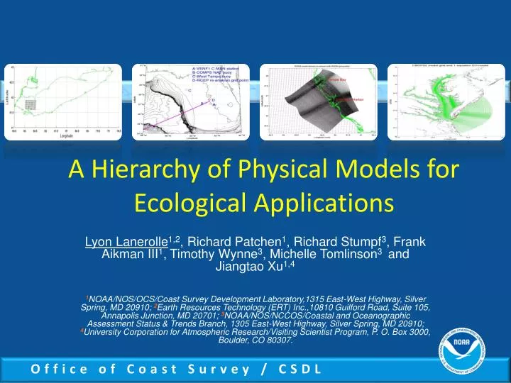
A Hierarchy of Physical Models for Ecological Applications

1. A Hierarchy of Physical Models for Ecological Applications Lyon Lanerolle1,2, Richard Patchen1, Richard Stumpf3, Frank Aikman III1, Timothy Wynne3, Michelle Tomlinson3 and Jiangtao Xu1,4 1NOAA/NOS/OCS/Coast Survey Development Laboratory,1315 East-West Highway, Silver Spring, MD 20910; 2Earth Resources Technology (ERT) Inc.,10810 Guilford Road, Suite 105, Annapolis Junction, MD 20701; 3NOAA/NOS/NCCOS/Coastal and Oceanographic Assessment Status & Trends Branch, 1305 East-West Highway, Silver Spring, MD 20910; 4University Corporation for Atmospheric Research/Visiting Scientist Program, P. O. Box 3000, Boulder, CO 80307.

2. Introduction and Motivation • Origin of modeling efforts due to research collaborations attempting to improve HAB and Hypoxia predictions: • 1D, 2D HAB set-ups due to NCCOS-CSDL collaboration • 3D HAB set-up due to NOAA/IOOS partnership project • Hypoxia set-up due to SURA Testbed (Estuarine Hypoxia) project • Hierarchy of modeling approaches due to : • Different levels of complexity of processes (e.g. 1D, 2D, 3D, etc.) • Nature of dominant physical processes (e.g. vertical mixing, upwelling, etc.) • All applications are physically forced usually with no behavior; all based on Rutgers University’s ROMS model • Modeling set-ups have dual purposes : (a) research tool and (b) real-time, operational forecast system (if needed)

3. 1D Vertical Mixing ModelMotivation and Model Set-up • Motivation: to study and predict cyanobacterial bloom/scum formation in water bodies • Model Design Specifications:(i) highly portable (speedily applied to any water body) and (ii) minimum number of model inputs – a simple grid, representative bathymetric value, a Coriolis parameter, a T and S profile for initialization and a fixed-point time-series of met. variables • Model set-up :ROMS with Bulk Fluxes, GLS k-ω closure, quadratic bottom drag (Cd=0.003), wall BCs, ∆t=300s (baroclinic) • Calibration :using idealized fields (thereafter applied to Western Lake Erie) • Computational Efficiency : 30-day simulation/per minute on LINUX box in serial mode (highly efficient) Acknowledgment : This work was funded by National Center for Environmental Health at the Centers for Disease Control and Prevention (CDC)

4. 1D Vertical Mixing ModelWestern Lake Erie Application and Results Marblehead, OH station • 9 x 9 horizontal grid • 20 vertical σ-levels • 7.7m flat bathymetry (from Obs.) • IC from linear interp. of a surface • and bottom T, S value • Met. forcing from NOAA/NDBC • Marblehead, OH station 1. Periods of high/low viscosity due to met. conditions 2. Simulated tracer and particles respond in the expected way

5. 2D Upwelling Transect ModelMotivation and Model Set-up • Motivation: Try to enhance WFS HAB event predictions of NOS/CO-OPS Bulletins by accounting for upwelling • Hypothesis: Upwelling contributes to HAB events on WFS • Model Design Specifications : Set-up model to study upwelling driven flow with cross-shore transport component • Model Set-up (ROMS): Grid : transect with 400 x 9 points, 80 vertical σ-levels Bathymetry : NOS soundings ICs : MODAS/Basin model (NGOM) for T and S and geostrophic velocities BCs : periodic and far-field radiation Forcings : met. forcing only (VENF1-CMAN and NAM) Vertical Mixing : GLS k-ω model Time Step : 150s (baroclinic)

6. 2D Upwelling Transect ModelModel Output and Results Particles respond to wind-driven upwelling (~31 August) • Algal cells simulated using Lagrangian particles (blue square – begin, blackcircle – end) • Model capable of running as Nowcast/Forecast system and generating above graphic • Computational Efficiency : 7-day simulation/hour or better on LINUX box in serial mode

7. 3D Nested/Coupled ModelMotivation and Modeling Strategy • Motivation : Try to enhance predictions of NOS/CO-OPS Bulletin HAB patch extent and movement on WFS - which is inherently 3D in nature • Model Design Specifications: Need a fully 3D model of WFS Need to include enough of shelf Need Tampa Bay and Charlotte Harbor Need to be computationally efficient • Modeling Strategy : Nest/Couple high-resolution ROMS model to already available basin-scale, POM-based NOAA/NOS Gulf of Mexico Model (NGOM)

8. 3D Nested/Coupled ModelModel Coupling and Set-up • Grid : Covers WFS and refined along coast, Tampa Bay and Charlotte Harbor; • 298 x 254 horizontal points and 30 vertical σ-levels • Bathymetry : NOS soundings (need to match at lateral boundaries) • Initial Conditions : NGOM interpolated water levels, T and S (spin-up from rest) • Boundary Conditions : NGOM interpolated surface forcings (wind stress, air P, heat flux); SST • correction; water levels, currents, T and S at lateral boundaries; tides from • ADCIRC added; 19 additional rivers (Tampa Bay and Charlotte Harbor) • ROMS details : Coupling BCs, Quadratic bottom drag, GLS k-ω model, ∆t=90 s (baroclinic) • Computational Efficiency : 24-day simulation/hour [MPI, IBM Power 6 cluster , 96 proc.] NGOM ROMS

9. 3D Nested/Coupled ModelModel Results Initialization HAB patch 7-day Hindcast Need 3D velocities as 2D depth-averaged velocities miss near-shore upwelling behavior Observed Initial Patch Digitized Initial Patch Tracer patch method : Passive/Inert tracer evolution within ROMS Particle tracking method : CSDL’s Chesapeake Bay Oyster Larvae Tracker (CBOLT)

10. Water Quality ModelMotivation and Model Set-up • Motivation : to study & predict spatio-temporal evolution of hypoxia in Chesapeake Bay • Strategy : begin with simplest WQ model and then build up to complex models • Model : examine hypoxia via DO using a 1-equation model with constant respiration (Malcolm Scully/ODU) • Model Set-up : embed DO model within NOAA/NOS Chesapeake Bay Operational Forecast System (CBOFS) DO in ROMS is a passive/inert tracer • Simulation : synoptic hindcast from June 01, 2003 - August 31, 2005 • ICs and BCs : DO saturation from T and S [Weiss (1970)]; no river DO sources • Computational Efficiency : 6-day sim./hour [MPI, IBM Power 6 cluster , 96 proc.] Const. resp. rate of 0.55 gO2/m3/day Fixed at saturation (surface also)

11. Water Quality ModelModel Results (Preliminary) DO ≤ 2 mg/L DO ≤ 1 mg/L DO ≤ 0.2 mg/L DO ≤ 2 mg/L at 1m above botm. • Total DO content (kg) diminishes during the summer months as expected • Hypoxic volumes show agreement with those derived from CBP observations* • Hypoxic zones present in deep, narrow channels during summer months *Courtesy of Malcolm Scully/ODU and Rebecca Murphy/JHU

12. Summary and Conclusions • Through collaborative efforts to study and predict (with improved accuracy) HABs and Hypoxia a suite of physical models have been developed at NOAA/NOS/OCS/Coast Survey Development Lab. • The models range in complexity depending on the nature of the dominant processes driving HABs and Hypoxia; they span multiple dimensions (1D - 3D) • Predictive capabilities of the models have been demonstrated and they reveal insights in to the driving physical mechanisms • These models, although developed as research tools, also have the potential to be cast in to Operational Forecast Systems (OFS) to routinely generate HAB and Hypoxia forecasts : http://tidesandcurrents.noaa.gov/hab/