4 Principal Component Analysis (PCA)

1. 4 Principal Component Analysis (PCA)

2. Intuition

3. Intuition (Continued)

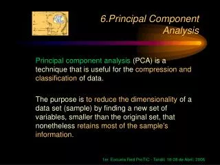
4. Principal Component Analysis • A method for re-expressing multivariate data. It allows the researchers to reorient the data so that the first few dimensions account for as much information as possible. • Useful in identifying and understanding patterns of association across variables.

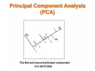
5. Principal Component Analysis • The first principal component, denoted Z1, is given by the linear combination of the original variables X=[X1,X2,…,Xp] with the largest possible variance. • The second principal component, denoted Z2, is given by the linear combination of X that accounts for the most information (highest variance) not already captured by Z1; that is, Z2 is chosen to be uncorrelated with Z1. • All subsequent principal components Z3, …, Zc are chosen to be uncorrelated with all previous principal components.

6. Mechanics Let z=Xu where X=[X1,X2,…,Xp], u=(u1,u2,…,up)’. Then, we have Var(z)=u’∑u where ∑=var(X). The problem thus can be stated as follows:

7. Mechanics (Continued) The Lagrangian is given by L=u’ ∑u-λ(u’u-1) where λ is called the Lagrange multiplier. Taking the deviative of L with respect to the elements of u yields

8. Eigenvalue-Eigenvector Equation ∑ u = λu where • the scalarλ is called an eigenvalue • the vector u is called an eigenvector • the square matrix ∑ is the covariance matrix of row random vector X, and can be estimated by the standardized data matrix Xsas follows:

9. Standardizing The Data Because principal component analysis seeks to maximize variance, it can be highly sensitive to scale difference across variables. Thus, it is usually (but not always) a good idea to standardize the data and denote them Xs. Example:

10. Principal Components (PCs) • Each eigenvector, denoted ui, represents the direction of the principal axes of the shape formed by the scatter plot of the data. The vector ui holds the weights used to form the linear combination of Xs that results in the principal component scores; that is, zi=Xsui. In matrix terms, Z=XsU. • Each eigenvalue, denoted λi, is equal to the variance of the principal component Zi. By design, the solution is chosen so that λ1≥ λ2≥… ≥λp≥0 • The covariance matrix for the princiapl components, denoted D, is a diagonal matrix with (λ1,λ2,… ,λp) on the diagonal. Thus, the standardized matrix of principal components is Zs=XsUD-1/2.

11. Principal Components (PCs) The sum of variances of all principal components is equal to p, the number of variables in the matrix X. Thus, the proportion of variation accounted for by the first c principal components is given by ?

12. Principal Component Loadings The correlation corr(X, Z) between the principal components Z and the original variables X F=UD1/2 The general expression for variance accounted for in variable Xi by the first c principal components is

13. PCA and SVD From the standardized matrix of principal components Zs=XsUD-1/2 We obtain Xs=ZsD1/2U’ What this reveals is that any data matrix X can be expressed as the matrix products of three simpler matrices. Zs is a matrix of uncorrelated variables, D1/2 is a diagonal matrix that performs a stretching transformation, and U’ is a transformation matrix that performs an orthogonal rotation. PCA=spectral decomposition of the correlation matrix /singular value decomposition of the data

14. When is it appropriate to use PCs? Bartlett’s Sphericity Test • Where • ln|R|=the natural log of the determinant of the correlation matrix • (p2-p)/2=the number of degrees of freedom associated with the chi-square test statistics • p=the number of variables • n=the number of observations

15. How many PCs should be retained There are several rules of thumb to be used in deciding the number of principal components to retain for further analysis: • The scree plot • Kaiser’s rule • Horn’s procedure

16. Example: Genetic Mapping

17. Example: Genetic Mapping (Cont’d)

18. Examples

19. Examples However, PCA doesnot necessarily preserve interesting information such as clusters.

20. Problems with Applications From “Nonlinear Data Representation for Visual Learning” by INRIA, France in 1998.

21. Non-linear PCA A simple non-linear extension of linear methods while keeping computational advantages of linear methods: • Map the original data to a feature space by a non-linear transformation • Run linear algorithm in the feature space

22. Example • d=2

23. Polar coordinate

24. Run PCA in feature space

25. Pull the results back to input space

26. PCA in Feature Space ■Centering in Feature Space:

27. PCA in Feature Space

28. PCA in High Dimensional Space (Dual Formulation)

29. PCA in High Dimensional Space (Dual Formulation, SVD)

30. PCA in High Dimensional Space (Dual Formulation, SVD)

31. PCA in High Dimensional Space (Dual Formulation)

32. PCA in High Dimensional Space (Dual Formulation)

33. Kernel PCA

34. Kernel PCA

35. Kernel PCA

36. Kernel PCA: Summary

37. Kernel PCA: An Example

38. Kernel PCA: An Example

39. Two-dimensional PCA (2DPCA) 2007年5月被引用次数：146 2008年5月被引用次数：339

41. 2DPCA

42. 2DPCA (Continued)

43. 2DPCA (Continued) m×d

44. Karhunen-Loeve Expansion

45. KL Expansion (Continued)

46. KL Expansion (Continued) KL Expansion = PCA

47. 小样本问题

48. Singular Value Decomposition(SVD) 奇异值分解定理 可以说明: U’U=I,即U的行是不相关的,方差为1.

49. 基于SVD的PCA变换

50. The ORL face databaseat the AT&T (Olivetti) Research Laboratory • The ORL Database of Faces contains a set of face images taken between April 1992 and April 1994 at the lab. The database was used in the context of a face recognition project carried out in collaboration with the Speech, Vision and Robotics Group of the Cambridge University Engineering Department. • There are ten different images of each of 40 distinct subjects. For some subjects, the images were taken at different times, varying the lighting, facial expressions (open / closed eyes, smiling / not smiling) and facial details (glasses / no glasses). All the images were taken against a dark homogeneous background with the subjects in an upright, frontal position (with tolerance for some side movement). • When using these images, please give credit to AT&T Laboratories Cambridge.