Lecture 4: Informed Heuristic Search

1. Lecture 4: Informed Heuristic Search ICS 271 Fall 2006

2. Summary • Heuristics and Optimal search strategies • heuristics • hill-climbing algorithms • Best-First search • A*: optimal search using heuristics • Properties of A* • admissibility, • monotonicity, • accuracy and dominance • efficiency of A* • Branch and Bound • Iterative deepening A* • Automatic generation of heuristics

3. Problem: finding a Minimum Cost Path • Previously we wanted an arbitrary path to a goal or best cost. • Now, we want the minimum cost path to a goal G • Cost of a path = sum of individual transitions along path • Examples of path-cost: • Navigation • path-cost = distance to node in miles • minimum => minimum time, least fuel • VLSI Design • path-cost = length of wires between chips • minimum => least clock/signal delay • 8-Puzzle • path-cost = number of pieces moved • minimum => least time to solve the puzzle

4. Heuristic functions • 8-puzzle • 8-queen • Travelling salesperson

5. Heuristic functions • 8-puzzle • W(n): number of misplaced tiles • Manhatten distance • Gaschnig’s • 8-queen • Travelling salesperson

6. Heuristic functions • 8-puzzle • W(n): number of misplaced tiles • Manhatten distance • Gaschnig’s • 8-queen • Number of future feasible slots • Min number of feasible slots in a row • Min number of conflicts (in complete assignments states) • Travelling salesperson • Minimum spanning tree • Minimum assignment problem

7. Heuristics E.g., for the 8-puzzle: • h1(n) = number of misplaced tiles • h2(n) = total Manhattan distance (i.e., no. of squares from desired location of each tile) • h1(S) = ? • h2(S) = ?

8. Heuristics E.g., for the 8-puzzle: • h1(n) = number of misplaced tiles • h2(n) = total Manhattan distance (i.e., no. of squares from desired location of each tile) • h1(S) = ? 8 • h2(S) = ? 3+1+2+2+2+3+3+2 = 18

9. Best first (Greedy) search: f(n) = number of misplaced tiles

10. Hill climbing, Greedy search • Example: • 8-queen, traveling salesperson, 8-puzzle, finding routes • Not systematic, • based on local optimization, memoryless, used by humans • Uses an heuristic evaluation function • that evaluates how far we are from the goal • Very greedy: • Expand current node and select the best among its children only if it is better than its own value until found a solution or reached a plateau. Keep only current node. • Greedy: • Expand current node and select the best among its children. Keep current path

11. Romania with step costs in km

12. Greedy best-first search • Evaluation function f(n) = h(n) (heuristic) • = estimate of cost from n to goal • e.g., hSLD(n) = straight-line distance from n to Bucharest • Greedy best-first search expands the node that appears to be closest to goal

13. Greedy best-first search example

14. Greedy best-first search example

15. Greedy best-first search example

16. Greedy best-first search example

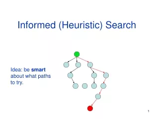
17. Problems with Greedy Search • Not complete • Get stuck on local minimas and plateaus, • Irrevocable, • Infinite loops • Can we incorporate heuristics in systematic search?

18. Informed search - Heuristic search • How to use heuristic knowledge in systematic search? • Where ? (in node expansion? hill-climbing ?) • Best-first: • select the best from all the nodes encountered so far in OPEN. • “good” use heuristics • Heuristic estimates value of a node • promise of a node • difficulty of solving the subproblem • quality of solution represented by node • the amount of information gained. • f(n)- heuristic evaluation function. • depends on n, goal, search so far, domain

19. A* search • Idea: avoid expanding paths that are already expensive • Evaluation function f(n) = g(n) + h(n) • g(n) = cost so far to reach n • h(n) = estimated cost from n to goal • f(n) = estimated total cost of path through n to goal

20. A* search example

21. A* search example

22. A* search example

23. A* search example

24. A* search example

25. A* search example

26. A*- a special Best-first search • Goal: find a minimum sum-cost path • Notation: • c(n,n’) - cost of arc (n,n’) • g(n) = cost of current path from start to node n in the search tree. • h(n) = estimate of the cheapest cost of a path from n to a goal. • Special evaluation function: f = g+h • f(n) estimates the cheapest cost solution path that goes through n. • h*(n) is the true cheapest cost from n to a goal. • g*(n) is the true shortest path from the start s, to n. • If the heuristic function, h always underestimate the true cost (h(n) is smaller than h*(n)), then A* is guaranteed to find an optimal solution.

27. A* on 8-puzzle with h(n) = w(n)

28. The Road-Map • Find shortest path between city A and B

29. Algorithm A* (with any h on search Graph) • Input: an implicit search graph problem with cost on the arcs • Output: the minimal cost path from start node to a goal node. • 1. Put the start node s on OPEN. • 2. If OPEN is empty, exit with failure • 3. Remove from OPEN and place on CLOSED a node n having minimum f. • 4. If n is a goal node exit successfully with a solution path obtained by tracing back the pointers from n to s. • 5. Otherwise, expand n generating its children and directing pointers from each child node to n. • For every child node n’ do • evaluate h(n’) and compute f(n’) = g(n’) +h(n’)= g(n)+c(n,n’)+h(n) • If n’ is already on OPEN or CLOSED compare its new f with the old f and attach the lowest f to n’. • put n’ with its f value in the right order in OPEN • 6. Go to step 2.

30. Best-First Algorithm BF (*) 1. Put the start node s on a list called OPEN of unexpanded nodes. 2. If OPEN is empty exit with failure; no solutions exists. 3. Remove the first OPEN node n at which f is minimum (break ties arbitrarily), and place it on a list called CLOSED to be used for expanded nodes. 4. Expand node n, generating all it’s successors with pointers back to n. 5. If any of n’s successors is a goal node, exit successfully with the solution obtained by tracing the path along the pointers from the goal back to s. 6. For every successor n’ on n:a. Calculate f (n’).b. if n’ was neither on OPEN nor on CLOSED, add it to OPEN. Attach a pointer from n’ back to n. Assign the newly computed f(n’) to node n’.c. if n’ already resided on OPEN or CLOSED, compare the newly computed f(n’) with the value previously assigned to n’. If the old value is lower, discard the newly generated node. If the new value is lower, substitute it for the old (n’ now points back to n instead of to its previous predecessor). If the matching node n’ resided on CLOSED, move it back to OPEN. • Go to step 2. * With tests for duplicate nodes.

31. B C A 10.4 6.7 4.0 11.0 G S 8.9 3.0 6.9 D F E 4 1 B C A 2 5 G 2 S 3 5 4 2 D F E

32. Example of A* Algorithm in action S 5 + 8.9 = 13.9 2 +10.4 = 12..4 D A 3 + 6.7 = 9.7 D B 4 + 8.9 = 12.9 7 + 4 = 11 8 + 6.9 = 14.9 6 + 6.9 = 12.9 E C E Dead End F B 10 + 3.0 = 13 11 + 6.7 = 17.7 G 13 + 0 = 13

33. Behavior of A - Termination • The heuristic function h(n) is called admissible if h(n) is never larger than h*(n), namely h(n) is always less or equal to true cheapest cost from n to the goal. • A* is admissible if it uses an admissible heuristic, and h(goal) = 0. • Theorem (completeness) (Hart, Nillson and Raphael, 1968) • A* always terminates with a solution path (h is not necessarily admissible) if • costs on arcs are positive, above epsilon • branching degree is finite. • Proof: The evaluation function f of nodes expanded must increase eventually (since paths are longer and costier) until all the nodes on an optimal path are expanded .

34. Behavior of A* - Completeness • Theorem (completeness for optimal solution) (HNL, 1968): • If the heuristic function is admissible than A* finds an optimal solution. • Proof: • 1. A* will expand only nodes whose f-values are less (or equal) to the optimal cost path C* (f(n) is less-or-equal C*). • 2. The evaluation function of a goal node along an optimal path equals C*. • Lemma: • Anytime before A* terminates there exists and OPEN node n’ on an optimal path with f(n’) <= C*.

35. Consistent (monotone) heuristics • A heuristic is consistent if for every node n, every successor n' of n generated by any action a, h(n) ≤ c(n,a,n') + h(n') • If h is consistent, we have f(n') = g(n') + h(n') = g(n) + c(n,a,n') + h(n') ≥ g(n) + h(n) = f(n) • i.e., f(n) is non-decreasing along any path. • Theorem: If h(n) is consistent, f along any path is non-decreasing. • Corollary: the f values seen by A* are non-decreasing.

36. Consistent heuristics • If h is monotone and h(goal)=0 then h is addimisible • Proof: (by induction of distance from the goal) • An A* guided by consistent heuristic finds an optimal paths to all expanded nodes, namely g(n) = g*(n) for any closed n. • Proof: Assume g(n) > g*(n) and n expanded along a non-optimal path. • Let n’ be the shallowest OPEN node on optimal path p to n  • g(n’) = g*(n’) and therfore f(n’)=g*(n’)+h(n’) • Due to monotonicity we get f(n’) <=g*(n’)+k(n’,n)+h(n) • Since g*(n) = g*(n’)+k(n’,n) along the optimal path, we get that • f(n’) <= g*(n) + h(n) • And since g(n) > g*(n) then f(n’) < g(n)+h(n) = f(n), contradiction

37. A* with consistent heuristics • A* expands nodes in order of increasing f value • Gradually adds "f-contours" of nodes • Contour i has all nodes with f=fi, where fi < fi+1

38. Summary of Consistent (Monotone) Heuristics • If in the search graph the heuristic function satisfies triangle inequality for every n and its child node n’: h(ni) less or equal h(nj) + c(ni,nj) • when h is monotone, the f values of nodes expanded by A* are never decreasing. • When A* selected n for expansion it already found the shortest path to it. • When h is monotone every node is expanded once (if check for duplicates). • Normally the heuristics we encounter are monotone • the number of misplaced ties • Manhattan distance • air-line distance

39. Admissible and consistent? heuristics E.g., for the 8-puzzle: • h1(n) = number of misplaced tiles • h2(n) = total Manhattan distance (i.e., no. of squares from desired location of each tile) • h1(S) = ? • h2(S) = ?

40. Admissible and consistent? heuristics E.g., for the 8-puzzle: • h1(n) = number of misplaced tiles • h2(n) = total Manhattan distance (i.e., no. of squares from desired location of each tile) • h1(S) = ? 8 • h2(S) = ? 3+1+2+2+2+3+3+2 = 18

41. Dominance • If h2(n) ≥ h1(n) for all n (both admissible) • then h2dominatesh1 • h2is better for search • Typical search costs (average number of nodes expanded): • d=12 IDS = 3,644,035 nodes A*(h1) = 227 nodes A*(h2) = 73 nodes • d=24 IDS = too many nodes A*(h1) = 39,135 nodes A*(h2) = 1,641 nodes

42. Summary of properties • A* expands every path along which f(n) < C* • A* will never expand any node s.t. f(n) > C* • If h is monotone A* will expand any node such that f(n) <C* • Therefore A* expands all the nodes for which f(n) < C* and a subset of the nodes for which f(n) = C*. • Therefore if h1(n) < h2(n) clearly the subset of nodes expanded is smaller.

43. Non-admissible heuristics:Adjust weights of g and h • F_w(n) = (1-w) g(n) +w h(n) • W = 0 (uniform cost) • W=1/2 (A*) • W=1 (DFS greedy) • If h is admissible then f_w is admissible for 0 <=w<=1/2

44. Complexity of A* • A* is optimally efficient (Dechter and Pearl 1985): • It can be shown that all algorithms that do not expand a node which A* did expand (inside the contours) may miss an optimal solution • A* worst-case time complexity: • is exponential unless the heuristic function is very accurate • If h is exact (h = h*) • search focus only on optimal paths • Main problem: space complexity is exponential • Effective branching factor: • logarithm of base (d+1) of average number of nodes expanded.

45. Effectiveness of A* Search Algorithm Average number of nodes expanded d IDS A*(h1) A*(h2) 2 10 6 6 4 112 13 12 8 6384 39 25 12 364404 227 73 14 3473941 539 113 20 ------------ 7276 676 Average over 100 randomly generated 8-puzzle problems h1 = number of tiles in the wrong position h2 = sum of Manhattan distances

46. Relationships among search algorithms

47. Pseudocode for Branch and Bound Search(An informed depth-first search) Initialize: Let Q = {S} While Q is not empty pull Q1, the first element in Q if Q1 is a goal compute the cost of the solution and update L <-- minimum between new cost and old cost else child_nodes = expand(Q1), <eliminate child_nodes which represent simple loops>, For each child node n do: evaluate f(n). If f(n) is greater than L discard n. end-for Put remaining child_nodes on top of queue in the order of their evaluation function, f. end Continue

48. B C A 10.4 6.7 4.0 11.0 G S 8.9 3.0 6.9 D F E 4 1 B C A 2 5 G 2 S 3 5 4 2 D F E

49. Example of Branch and Bound in action S 2 5 D A

50. Properties of Branch-and-Bound • Not guaranteed to terminate unless has depth-bound • Optimal: • finds an optimal solution • Time complexity: exponential • Space complexity: linear